Defining the Pipeline

Section overview

In this section, we cover creating our basic pipeline, which will use a multi-class Support Vector Machine (SVM) to classify the data. Later on in the tutorial, we will experiment with different solutions, and learn how each variation affects the metrics we are tracking.

Our pipeline will consist of the following stages:

1. Import training and test data.
   • Output: The train and test splits of the data.
2. Featurization or pre-processing.
   • Output: Processed data, ready for model training.
3. Training, in which our model is created and trained base on the training dataset.
   • Output: The trained model, plus training metrics.
4. Evaluation, in which our model is scored for performance on the testing dataset.
   • Output: Metrics for our model's performance on the test data.

We have chosen two metrics which will be measured throughout our pipeline - the model training time and test accuracy. They are not necessarily the "correct" metrics for a project like this, but are used mainly to show how DVC works with metrics.

DVC uses the command dvc run in order to create stages in the pipeline. A stage is defined by its dependencies, outputs and metrics, as well as the command needed to reproduce the stage. We will see examples for many of these in this tutorial.

Importing the data

We'll use the MNIST datasets in CSV format, as prepared by https://pjreddie.com.

We'll go over two ways to add the data to your code. The most straightforward way is using the dvc import-url command.

dvc import-url https://pjreddie.com/media/files/mnist_train.csv data/train_data.csv
dvc import-url https://pjreddie.com/media/files/mnist_test.csv data/test_data.csv

This will download the file directly from the url and begin tracking it using DVC. Another way is to download the files to your project folder using curl and then use dvc add to track them.

curl https://pjreddie.com/media/files/mnist_train.csv -o data/train_data.csv
curl https://pjreddie.com/media/files/mnist_test.csv -o data/test_data.csv

dvc add data/train_data.csv
dvc add data/test_data.csv

Info

dvc add is similar to git add - it tells DVC that this is a file we should be tracking changes on. The immediate effect of this command will be that the file is added to .dvc/cache

Committing progress to Git

Lets check the Git status of the data folder.

Linux/MacWindows

$ git status -s
?? data/

$ git status -s data/*
?? data/.gitignore
?? data/test_data.csv.dvc
?? data/train_data.csv.dvc

$ cat data/.gitignore
/train_data.csv
/test_data.csv

$ git status -s
?? data/

$ git status -s data/*
?? data/.gitignore
?? data/test_data.csv.dvc
?? data/train_data.csv.dvc

$ type data\.gitignore
/train_data.csv
/test_data.csv

As you might have noticed, the data files themselves (which weigh around 130Mb together) are not tracked by Git. Adding them to the .gitignore file is part of the dvc import-url and dvc add command. What these commands additionally do, is keep the actual file in the DVC cache located in .dvc/cache and create a reflink to the file in its intended location in data/. This means that in practice you don't use twice the space, which is a pretty neat feature.

Now, to commit the changes:

git add .
git commit -m "Imported training and test datasets"
git push
dvc push -r origin

Info

Similar to git push, dvc push deploys changes; only to the data files within the repository! Our data files are pushed to the remote, and can be accessed via the dagshub repository.

Visualizing changes

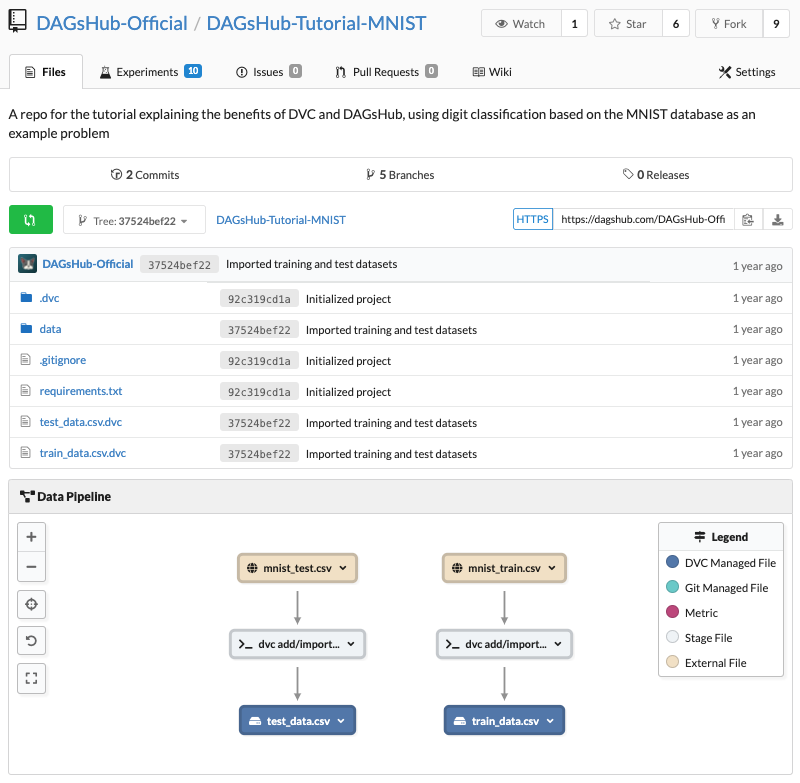
Let's go back to our repo page and see how it looks now.

_{Repo view after importing data}
Surprise! we have a DAG with 6 nodes appearing in the Data Pipeline view. Let's dive into the meaning and uses of each node.

The first node is the remote location we imported the data from. If we click on it it expands and we can see the following details:

_{Data node}
The Yellow color signifies that this is a generic untracked file node, which is usually data but could be normalization parameters or anything that doesn't fall into any of the other file categories.

The rest of the data represented by this node is as follows:

1. Icon representing the file location. In our case, the file is downloaded from the internets, and therefore we have a globe icon.
2. The file name.
3. Path to the file, in the case of http/s, this is a clickable link to the file's original location.
4. The location of the file in textual form.

The lower files are the same as these, but represent the data files that are now in our project. Since the working copy is located on our machine, they have an HDD icon, and if you expand them, the path link is disabled due to the fact that they are not available online (Remember, they are not committed to git!). We will solve this in the optional stage Adding a Remote Cache at the end of this section.

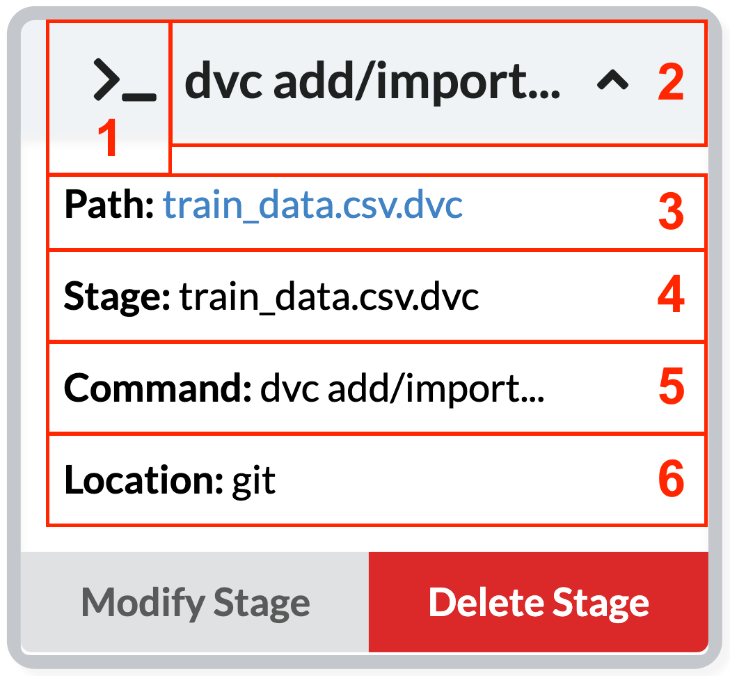
The nodes in the middle are stage nodes (or nodes representing .dvc files). Let's expand one and see what details they hold:

_{DVC node}
Here, the gray color represents that this is a stage node, meaning it describes a stage in the pipeline.

The other details represent the following:

1. In the case of stage nodes, the icon is a terminal icon, representing that this is a command. It's pointless to show a location icon, since .dvc files are always checked into the git repo.
2. The command that created this stage. We may truncate it if it's too long. In this case, the command is just a dvc add or import. Later in the tutorial, we will see stages where the command is more complex and defined by the user.
3. Path to the DVC file containing the details of the command. You can click on it to see the contents of the file in your browser.
4. The name of the stage - in this case the stage is named after the .dvc filename created by the dvc import command.
5. The full command used to create the stage. Not much info here in the case of dvc add or import.
6. Location of the dvc file. Should always be Git.

Now let's move on to create the rest of the pipeline.

Featurization or pre-processing

First, we need to create a python module to pre-process our data. You can download it from this link and save it to your code/ folder as featurization.py.

Here is the code:

"""
Create feature CSVs for train and test datasets
"""
import json
import numpy as np
import pandas as pd


def featurization():
    # Load data-sets
    print("Loading data sets...")
    train_data = pd.read_csv('./data/train_data.csv', header=None, dtype=float)
    test_data = pd.read_csv('./data/test_data.csv', header=None, dtype=float)
    print("done.")

    # Normalize the train data
    print("Normalizing data...")
    # We choose all columns except the first, since that is where our labels are
    train_mean = train_data.values[:, 1:].mean()
    train_std = train_data.values[:, 1:].std()

    # Normalize train and test data according to the train data distribution
    train_data.values[:, 1:] -= train_mean
    train_data.values[:, 1:] /= train_std
    test_data.values[:, 1:] -= train_mean
    test_data.values[:, 1:] /= train_std

    print("done.")

    print("Saving processed datasets and normalization parameters...")
    # Save normalized data-sets
    np.save('./data/processed_train_data', train_data)
    np.save('./data/processed_test_data', test_data)

    # Save mean and std for future inference
    with open('./data/norm_params.json', 'w') as f:
        json.dump({'mean': train_mean, 'std': train_std}, f)

    print("done.")


if __name__ == '__main__':
    featurization()

The code loads the training and test datasets using pandas, normalizes them, saves them as .npy files, and saves the normalization parameters in a separate .json file. We'll need those later, for inference in production.

A few things to note

• It is important to note file names. The processed data files will be saved as processed_train_data.npy and processed_test_data.npy and the normalization parameters will be saved as norm_params.json. This is important as we'll use these as arguments for the dvc run command.

Now, to create the stage and run the code, use the following command:

Linux\MacWindows

dvc run -n featurization\
-d data/train_data.csv \
-d data/test_data.csv \
-d code/featurization.py \
-o data/norm_params.json \
-o data/processed_train_data.npy \
-o data/processed_test_data.npy \
python3 code/featurization.py

dvc run -n featurization ^
-d data/train_data.csv ^
-d data/test_data.csv ^
-d code/featurization.py ^
-o data/norm_params.json ^
-o data/processed_train_data.npy ^
-o data/processed_test_data.npy ^
python3 code/featurization.py

The -n specifies how to name the stage resulting from this dvc run command. It is a good practice to give it a descriptive name.

The -d flags define dependencies of the stage, and include both data and code files (in our case).

The -o files define cached outputs. This means that after running the command, DVC will cache these files in .dvc/cache and track their changes (as well as add them to .gitignore). A file specified with -o needs to be generated by the command in question.

Uncached outputs

DVC also enables you to define uncached outputs with the -O flag. These files will be tracked by Git instead of living in the .dvc/cache.

The last line is the command itself. It is possible to input any shell command as the dvc command.

Every dvc run command creates a dvc.yaml file and a dvc.lock file. Let's look at the contents of these file:

$ cat dvc.yaml
stages:
  featurization:
    cmd: python3 code/featurization.py
    deps:
    - code/featurization.py
    - data/test_data.csv
    - data/train_data.csv
    outs:
    - data/norm_params.json
    - data/processed_test_data.npy
    - data/processed_train_data.npy

This file holds details on the stage, including the command which you can see in the Data Pipeline view, as well as the dependencies and outputs. From now on whenever you'll run dvc run, a new stage with its dependencies and outputs will appear in this file.

Now let's look at dvc.lock:

$ cat dvc.lock
featurization:
  cmd: python3 code/featurization.py
  deps:
  - path: code/featurization.py
    md5: e570a5b45022e46e9d6ad9cd6f2a1887
  - path: data/test_data.csv
    md5: c807df8d6d804ab2647fc15c3d40f543
  - path: data/train_data.csv
    md5: 5b49cf1b57fb9d6102b559d59d99df7c
  outs:
  - path: data/norm_params.json
    md5: e46984ac8b7097bfddfe5d9210f78ca4
  - path: data/processed_test_data.npy
    md5: a5257a91e73920bdd4cafd0f88105b74
  - path: data/processed_train_data.npy
    md5: 9ee0468925c998fda26d197a14d1caec

For every one of the stages appearing in dvc.yaml a record exists in this file too. The difference is that a md5 hash is saved for every dependency and output. Every time you will want to run this stage, dvc will compare the current md5 of the files on your system to the ones in this file, and determine if the pipeline stage should be re-run. Examples will come later in the tutorial.

Let's perform another step before committing to Git.

Model training

After processing our data, we now wish to train a multiclass SVM on the training data. We will create a file called code/train_model.py. You can download the complete file from this link.

Here is the code:

"""
Train classification model for MNIST
"""
import json
import pickle
import numpy as np
from sklearn.svm import SVC
from sklearn.multiclass import OneVsRestClassifier
import time


def train_model():
    # Measure training time
    start_time = time.time()

    # Load training data
    print("Load training data...")
    train_data = np.load('./data/processed_train_data.npy')

    # Choose a random sample of images from the training data.
    # This is important since SVM training time increases quadratically with the number of training samples.
    print("Choosing smaller sample to shorten training time...")
    # Set a random seed so that we get the same "random" choices when we try to recreate the experiment.
    np.random.seed(42)

    num_samples = 5000
    choice = np.random.choice(train_data.shape[0], num_samples, replace=False)
    train_data = train_data[choice, :]

    # Divide loaded data-set into data and labels
    labels = train_data[:, 0]
    data = train_data[:, 1:]
    print("done.")

    # Define SVM classifier and train model
    print("Training model...")
    model = OneVsRestClassifier(SVC(kernel='linear'), n_jobs=6)
    model.fit(data, labels)
    print("done.")

    # Save model as pkl
    print("Save model and training time metric...")
    with open("./data/model.pkl", 'wb') as f:
        pickle.dump(model, f)

    # End training time measurement
    end_time = time.time()

    # Create metric for model training time
    with open('./metrics/train_metric.json', 'w') as f:
        json.dump({'training_time': end_time - start_time}, f)
    print("done.")


if __name__ == '__main__':
    train_model()

The code loads the processed training data file, divides into data and labels, takes a smaller subsample to maintain reasonable training times, and trains a Scikit-Learn multiclass SVM on it. All the while we measure the training time, as we would like to keep it low (We don't want to waste your time while going through this tutorial    ∩(︶▽︶)∩   ).

Now, let's run the training stage:

Linux\MacWindows

dvc run -n training \
-d data/processed_train_data.npy \
-d code/train_model.py \
-M metrics/train_metric.json \
-o data/model.pkl \
python3 code/train_model.py

dvc run -n training ^
-d data/processed_train_data.npy ^
-d code/train_model.py ^
-M metrics/train_metric.json ^
-o data/model.pkl ^
python3 code/train_model.py

Here, we have a new flag -M which tells DVC to mark the following file as a metric. Metric files are expected to be small and will be checked into git rather than being tracked by DVC. In DVC jargon, they will be uncached.

Committing to Git

Let's check the Git status of the data folder.

$ git status -su
M data/.gitignore
?? code/featurization.py
?? code/train_model.py
?? dvc.lock
?? dvc.yaml
?? metrics/train_metric.json

We now have two new dvc files representing our two pipeline stages, as well as the two code files, one for each stage. The metric file will be committed to git as well.

The .gitignore file has been updated to include the DVC tracked files:

Linux/MacWindows

$ cat data/.gitignore
/train_data.csv
/test_data.csv
/norm_params.json
/processed_train_data.npy
/processed_test_data.npy
/model.pkl

$ type data\.gitignore
/train_data.csv
/test_data.csv
/norm_params.json
/processed_train_data.npy
/processed_test_data.npy
/model.pkl

Now, to commit the changes:

git add .
git commit -m "Trained basic multiclass SVM model"
git push

Visualizing changes

First, it's worth noting that in order to view metrics in the command line, you can use the built in command:

$ dvc metrics show
    metrics/train_metric.json:
        training_time: 11.965423107147217

So we know that training has taken a bit less than 12 seconds. We think that's a reasonable time for this tutorial.

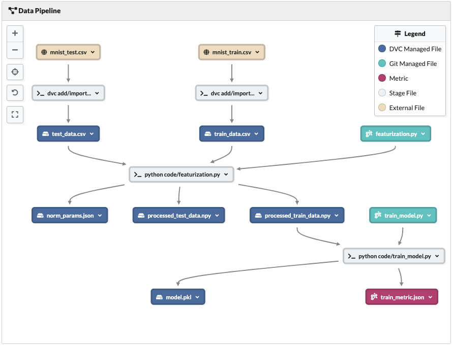
Let's go back to our repo page and see how our data pipeline looks now.

_{Data Pipeline view after processing data and training model} Now THAT is a DAG ()! Let's quickly go over the flow of our pipeline:

1. We imported the data from an online https:// address and tracked it locally.
2. Using featurization.py we took that data and processed it, outputting the processed data as .npy files and a normalization parameters .json file.
3. We then used our next block of code train_model.py and processed_train_data.npy to train an SVM model, while measuring the training time and tracking it as a metric.

That's it. There are three stages, represented by three stages in dvc.yaml.

We also have two new types of nodes.

The first is a code node. When expanded we get:

_{Code node}
The only new thing here is the green color which represents that this is a code file.

The red file represents a metric node:

_{Metric node}

Let's create the final stage of our pipeline.

Evaluating the model

For the evaluation stage we have decided to use the accuracy metric. DVC gives you complete freedom in choosing your metrics, and will display metric details properly as long as they are defined in the same way throughout your project.

We will call the evaluation module eval.py You can download the code from this link and put it in your code folder.

This is the code:

"""
Evaluate model performance
"""
import pickle
import json
import numpy as np
from sklearn.metrics import accuracy_score, precision_score, recall_score, roc_auc_score


def eval_model():
    # Load test data
    print("Loading data and model...")
    test_data = np.load('./data/processed_test_data.npy')

    # Load trained model
    with open('./data/model.pkl', 'rb') as f:
        model = pickle.load(f)
    print("done.")
    # Divide loaded data-set into data and labels
    labels = test_data[:, 0]
    data = test_data[:, 1:]

    # Run model on test data
    print("Running model on test data...")
    predictions = model.predict(data)
    print("done.")

    # Calculate metric scores
    print("Calculating metrics...")
    metrics = {'accuracy': accuracy_score(labels, predictions)}

    # Save metrics to json file
    with open('./metrics/eval.json', 'w') as f:
        json.dump(metrics, f)
    print("done.")


if __name__ == '__main__':
    eval_model()

Now let's use the last DVC run command for this pipeline to create the evaluation stage:

Linux/MacWindows

dvc run -n eval \
-d data/processed_test_data.npy \
-d data/model.pkl \
-d code/eval.py \
-M metrics/eval.json \
python3 code/eval.py

dvc run -n eval ^
-d data/processed_test_data.npy ^
-d data/model.pkl ^
-d code/eval.py ^
-M metrics/eval.json ^
python3 code/eval.py

Now, let's see what our model's accuracy score is?

$ dvc metrics show
Path                       accuracy    training_time
metrics/train_metric.json  -           62.85439
metrics/eval.json          0.9845      -

We can see that the resulting model's accuracy is 98%. Pretty neat for a minute of training!

---

Committing to Git

Lets check the Git status of the data folder.

$ git status -s
 M dvc.yaml
 M dvc.lock
?? code/eval.py
?? metrics/eval.json

We have the new files created by the evaluation stage, as well as modified dvc.yaml and dvc.lock files resulting from adding a stage.

Now, to commit the changes:

git add .
git commit -m "Evaluate basic SVM model"
git push
dvc push -r origin

We run dvc push once again to push our newly generated data - here, the model's parameters, the model itself and processed datasets - to dagshub cloud storage.

Visualizing changes

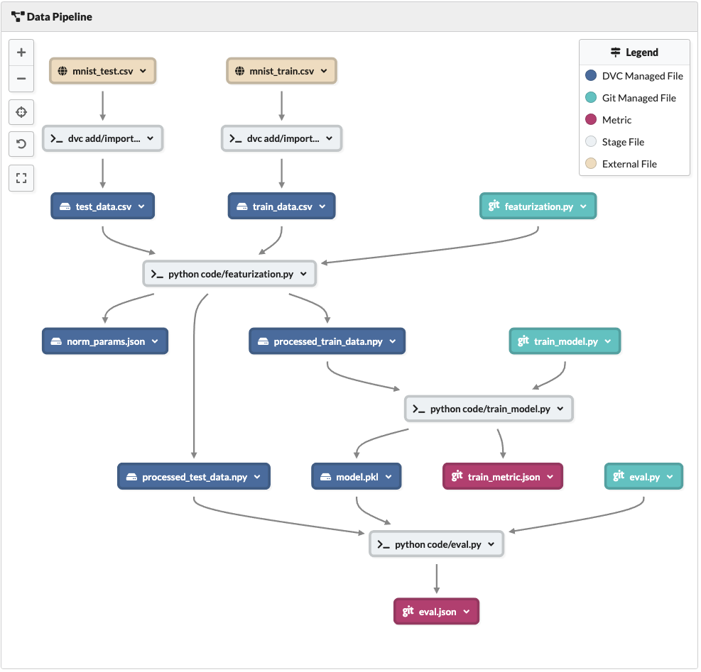
Our pipeline is now complete and should look like this in the Data Pipeline view:

_{Data Pipeline view after processing data and training model}

As we can see the eval.py code file, as well as the model.pkl and processed_test_data.npy are used as dependencies for the last stage. The last stage outputs a new metric file eval.json which holds the accuracy metric.

The "hard" task of setting up the pipeline is done, and we can now move onto experimenting and reaping the benefits of this setup. This is what we'll do in the next section.

You can also complete this next stage, which covers adding a remote cache. This is extremely important for team collaboration, and requires some remote storage account. If this is relevant to you, we recommend not to skip it.

---

Optional - adding a remote cache

Throughout this tutorial, we have used Git to version and share our code files as well as the dvc stage files that have been created throughout our pipeline. The code managed by Git has been pushed to our Git remote (hosted on dagshub.com), but the data files managed by DVC are still on our local machine, in the .dvc/cache.

DVC, however, enables you to push your data and models to the cloud, and thus to share them with team members and collaborators. Just like pushing your code to a shared Git remote enables you to share code with your team mates.

We will cover how to do that, using Google Storage (the cloud storage service, not to be confused with Google Drive). The same methods with very slight modifications will work with other cloud providers, such as AWS and Azure, and even with just plain old shared directories or SSH servers.

We assume that you have already created a storage bucket for this tutorial, have the appropriate permissions and the URL for it.

In our case we have called the bucket dagshub-tutorial and the link is gs://dagshub-tutorial. You will have viewing permission for our bucket but won't be able to push files to it.

To push our data to a remote cache, we need to do a few things:

Installing the DVC extension

Install the corresponding dvc remote. If you have the command line utility for the cloud service you are using, you can skip this step. Otherwise type in the following command (according to the service you are using):

All Extensions

pip3 install 'dvc[all]'

AWS - Amazon Web Services

pip3 install 'dvc[s3]'

GS - Google Storage

pip3 install 'dvc[gs]'

Microsoft Azure

pip3 install 'dvc[azure]'

SSH

pip3 install 'dvc[ssh]'

After the installation reopen the terminal window to make sure the changes have taken place.

Defining the remote in DVC

Define the dvc remote. We do this with one command (don't forget to replace the bucket name with your own bucket):

dvc remote add --local gs_remote gs://dagshub-tutorial

As long as you don't forget the --local flag, this shouldn't affect your Git repo. You can confirm this by running git status and seeing that there are no uncommitted changes

Why --local?

It is our opinion that the configuration of the remote may vary between team members (working in various environments) and over time (if you switch between cloud providers), therefore it is prudent not to modify the .dvc/config file which is monitored by Git.

Instead, we prefer to use the local configuration instead. You can find it in .dvc/config.local, and confirm that it's ignored in .dvc/.gitignore.

That way you don't couple the current environment configuration to the code history. This is the same best practice which naturally occurs when you run git remote add - the configuration is only local to your own working repo, and won't be pushed to any git remote.

Pushing the files to the cloud

Is as simple as one command.

dvc push -r gs_remote

This step might take a while.

Profit!

To reap the benefits of doing this while using DagsHub to host your repo, go to your repo settings, and add the link to the bucket in the Advanced Settings Local DVC cache URL. In our case it looks something like this:

_{Local DVC cache URL setting}

Going back to the nodes that were locally stored, they now have functioning links, and are therefore available for viewing or download for anyone who would want to (provided they have authorization to your bucket, of course).


_{Path link change after adding remote}

We believe this is useful for several reasons:

• If you want to let someone browse your data and trained models, you can just send them a link to your DagsHub repo. They don't need to clone or run anything, or sift through undocumented directory structures to find the model they are looking for.
• The files managed by DVC and pushed to the cloud are immutable - just like a specific version of a file which is saved in a Git commit, even if you continue working and the branch has moved on, you can always go back to some old branch or commit, and the download links will still point to the files as they were in the past.
• By using DVC and DagsHub, you can preserve your own sanity when running a lot of different experiments in multiple parallel branches. Don't remember where you saved that model which you trained a month ago? Just take a look at your repo, it's a click away. Let software do the grunt work of organizing files, just like those wonderfully lazy software developers do.

Warning

When downloading a link through the graph, it might be saved as a file with the DVC hash as its filename. You can safely change it to the intended filename, including the original extension and it'll work just fine.

Additionally you can use the dvc pull command to retrieve the remote data, which was possibly pushed there by someone else.

dvc pull -r gs_remote

---

Congratulations on building your first DagsHub/DVC pipeline. Let's experiment with it and see how DVC enables reproducibility, in the next section.