Querying and saving subsets of your datasets

Using the automatically generated enrichments, or the ones you manually added previously, Data Engine provides the ability to zoom in and focus on relevant data points by querying your data source and generating new subsets to train your model on.

There are 2 ways to query your data source:

1. Using the Python Client API
2. Using the Web UI

1. Client API Queries

Data Engine queries are structured in a familiar Pandas-like syntax.

A few query examples:

# Get all data points from episodes after 5
q1 = ds["episode"] > 5

# Get all data points from the first episode that also include baby Yoda in them 
q2 = (ds["episode"] == 1) & (ds["has_baby_yoda"] == True)

# Get data points that aren't between episodes 4 and 6
q3 = ~((ds["episode"] >= 4) & (ds["episode"] <= 6))

# Get data points that don't have an attached annotation
q4 = ds["annotation"].is_null()

Filtering operators

Data Engine supports the following operators:

• == (equal)
• != (not equal)
• > (greater than)
• >= (greater than or equal)
• < (less than)
• <= (less than or equal)
• .is_null()
• .is_not_null()
• Filters applicable to string fields:
  • .contains("value")
  • .startswith("startval")
  • .endswith("endval")
• Filters applicable to datetime fields:
  • .date_field_in_timeofday("10:00-14:00") - any date with time in between 10:00 and 14:00
  • .date_field_in_days(1, 2, 3) - any date where the day number is 1, 2, or 3
  • .date_field_in_months(1, 2) - any date in the months of January and February
  • .date_field_in_years(2020, 2022) - any date in years 2020 or 2022
  • .with_time_zone("+03:00") - explicitly set the timezone offset for the query, all datetime comparisons will be done relative to this offset.
• For composing multiple queries together:
  • & (and)
  • | (or)
  • ~ (not)

The query composition operators (&, |, ~) are binary and will be executed before the regular operators. For example:

# Supported
new_ds = (ds["episode"] > 5) & (ds["has_baby_yoda"] == True)

# Not supported
new_ds = ds["episode"] > 5 & ds["has_baby_yoda"] == True 

Notes and limitations:

1. Comparison is supported only on primitives - comparison between columns is not supported yet.
2. The in, and, or, not syntax (Python) is not supported. Usecontains(), &, | , ~ instead. For example:

   # Supported
   ds["col"].contains("aaa")
   ds = (ds["episode"] == 0) & (ds["has_baby_yoda"] == True)
   ds[~(ds["episode"] == 0)]
   
   # Not supported
   "aaa" in df["col"]
   ds = (ds["episode"] == 0) and (ds["has_baby_yoda"] == True) 
   

3. For re-querying, assign the result to a new variable to not lose the query. For example:

   # Supported
   filtered_ds = ds[ds["episode"] > 5]
   filtered_ds2 = filtered_ds[filtered_ds["has_baby_yoda"] == True]
   
   # Not supported 
   filtered_ds = ds[ds["episode"] > 5]
   filtered_ds2 = filtered_ds[ds["has_baby_yoda"] == True]
   

4. .with_time_zone() applies to the whole query, every new application will overwrite the previous:

   ds1 = ds["taken_at"].date_field_in_timeofday("10:00-12:00)
   ds2 = ds["taken_at"].date_field_in_days(5, 6).with_time_zone("+03:00")
   ds3 = ds1 & ds2    # Will look for 10:00-12:00 in UTC+3 offset!!!
   

Example of using datetime filtering to get datapoints with the value of taken_at older than 2024-06-01, in between 10:00 and 14:00, with UTC-5 offset (EST):

dt_start = datetime.datetime(2024, 6, 1)
queried = (ds["taken_at"] > dt_start)["taken_at"].date_field_in_timeofday("10:00-14:00").with_time_zone("-05:00")
res = queried.all()

Selecting metadata columns

Using select() you can choose which columns will appear in your query result and what their names will be (alias). For example:

q1 = (ds["size"] > 5).select("path", "size")

Will return all datapoints with size greater than 5, only the 2 columns selected, and not any other column in the dataset's enrichments.

Notes and limitations:

1. The path, datapoint_id, and dagshub_download_url columns will always be returned, as they are needed for Data Engine functionality
2. Both "x" and Field("x") can be used
3. alias, as_of - are optional
4. We currently do not check the list for contradictions/overwrites/duplications, i.e. select("x","x") or select(Field("a", alias="X"), Field("b", alias="X")) would not make much sense. however, if you provide a 'as_of' but do not provide an alias, the results will be auto-aliased in the form: "xxx_as_of_2023_12_11_14_42_20_UTC" where xxx is the column name.

Versioning filters

Datasource's and dataset's enrichments are versioned, and you can return to the state of a certain metadata field or an entire datasource to a previous point in time. To do this easily, we provide a few versioning filters

A simple example uses the global as_of time filter looks like this:

from datetime import *
t_prev = datetime.now() - timedelta(hours=24)
ds_v1 = ds.as_of(t_prev)

Filtering queries by previous versions

An extended syntax lets you query according to different versions of enrichments. For example:

# these includes are required for the bellow 4 snippets
from datetime import datetime, timezone, timedelta
from dagshub.data_engine.model.datasource import Field

# size metadata is constantly changed and we want to address the one from 24h ago
t = datetime.now(timezone.utc) - timedelta(hours=24)

q1 = ds[Field("size", as_of=t)] > 5

In the above example all datapoints whose "size" column was updated no later than 't' that match the condition '>5' are returned.

Query select with previous versions

Using select() also works with the as_of argument in the Field function, meaning you can select multiple versions of the same column to view, for example 2 versions of the annotation column might be valuable to visually compare them and decide which one is better. Similarly, you might want to compare to model prediction versions to visually inspect model performance.

t = datetime.now(timezone.utc) - timedelta(hours=24)

q1 = (ds["size"] > 5).select(Field("size", as_of=t, alias="size_asof_24h_ago"), Field("episode"))

In the above example the result set of datapoints will have 2 columns of metadata: "size_asof_24h_ago" and "episode". all other metadata columns are ommited.if the desired result is to get all metadata columns and in addition the selected list, add "*" to the list, example:

q1 = (ds["size"] > 5).select(Field("size", as_of=t, alias="size_asof_24h_ago"), "*")

Global as_of time

Using as_of() applied on a query allows you to view a snapshot of datapoint/enrichments. For example:

t = datetime.now(timezone.utc) - timedelta(hours=24)

q1 = (ds["size"] > 5).as_of(t)

in the above example all datapoints whose creation time is no later than 't' and that match the condition at 't' - are returned.

Notes and limitations:

Time parameter - the time parameter can be POSIX timestamp or datetime object - pay attention to timezones - use timestamp if known, or relative datetime if known (as in the above examples). if you use a specific date such as dateutil.parser.parse("Tue 28 Nov 11:29 +2:00") specify the utc delta as shown here, otherwise this date can translate to different timestamps in the machine that runs the client and in dagshub backend.

Global as_of behavior - it applies to all entities unless otherwise specified, i.e if we use Field("x", as_of=t1)) then t1 will precede over a t2 specified in .as_of(t2). the sensibility of the results is up to the caller. you could get datapoints that existed in t1 < t2 based on a condition applied on their enrichments in t2.

Creating DataFrames from query results

Use .dataframe to get a pandas DataFrame that contains the data points and their enrichments:

df = ds.head().dataframe

# You can also use it like this
ds[ds["episode"] > 5].all().dataframe

Note

.dataframe provides a copy of the metadata as a DataFrame. Changes made on a DataFrame do not apply to the original data source it was created from.

Saving query results as a new dataset

Query results can be saved and used later as a new dataset. To save your results as a new dataset, use the .save_dataset function:

# Filtered datasource
new_ds = ds[["episode"] > 5]

# Save the query as a dataset
new_ds.save_dataset("dataset-name")

After saving the new dataset, it will be displayed in your repository under the Datasets tab:

To get a list of all the saved datasets in a repository, use the get_datasets function:

from dagshub.data_engine import datasets
ds_list = datasets.get_datasets("username/repoName")

View and use saved datasets

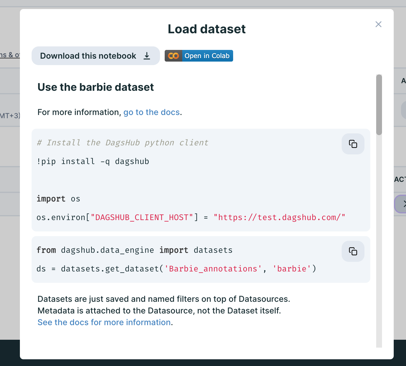
To use saved datasets, use the .get_dataset() function:

from dagshub.data_engine import datasets

ds = datasets.get_dataset("user/repo", "dataset-name")

Or navigate to the datasets tab in your repository, click on the Use this dataset button attached to the relevant dataset, and follow the instructions:

Where you'll see a notebook full of copyable code snippets enabling you to use your dataset:

2. Using the Web UI

You can access the query editor at the banner above the datapoints once you select your datasource or dataset.

The intuitive setup of the query builder is similar to that of the queries passed through the Python client: applying any query results in your_query.all() being run server-side, rendering filtered datapoints from the QueryResult.

Basic Queries

By default, queries are sets of AND conditions. Datapoints that evaluate to true for every condition are returned. For example, in the Sawit dataset project, to find the birds annotated by humans in the test split, you can:

1. Select + to add a condition.
2. Choose key 'split' and check if it is equal to 'test': split == 'test'.
3. Add another condition, this time to check if annotator is human: annotator == 'human'visualizing_datasets/#save-query-results-as-a-dataset.
4. Hit Apply Query.
5. Optionally, save it as a new dataset.

Advanced Queries

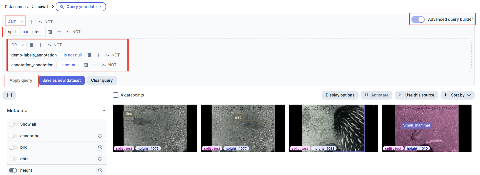
Of course, there are cases where chaining conditions with AND is simply not enough. In this case, we need to use the advanced query builder. It allows us to build queries with the same expressivity as the Client API!

Going back to the Sawit project, we can see that our metadata consists of annotations by two separate LabelStudio annotation projects. We can connect these two with an OR clause:

1. Select + to add a condition.
2. Choose key 'demo-labels_annotation', and hit NOT to query non-null values.
3. Carry out the same process for 'annotations_annotation'.
4. Change the condition operator to OR.
5. Hit Apply Query.

Info

The dotted/solid outlines highlight a 'condition group', a visualization of: (<operand> <OR/AND> <operand>). An operand in this context is anything that evaluates to true or false, and so can be a condition group in itself or just a single condition.

We can use condition groups to set up more complex actions. For instance, to identify just the annotated datapoints within the test split, we can create a 'annotations' condition group and a 'split' condition group.

1. Select + to add a condition group.
2. Carry out the steps from the previous query to create the OR condition group that identifies annotations from either group.
3. Select + at the root level and create a condition.
4. Choose key 'split' and check if it is equal to 'test': split == 'test'.
5. Hit Apply Query.

Sorted Order

We can render the datapoints in sorted order by specifying a hierarchy of columns and whether the column should be sorted in increasing or decreasing order.

Display Options

From the bar above your datapoints, you can also select Display Options. Here’s what they all do:

1. Show labels: Whether or not the labels from LabelStudio should be overlaid over datapoint.
2. Show bounding boxes: Whether or not the bounding boxes from LabelStudio should be overlaid over each datapoint.
3. Show filenames: Whether or not filenames should overlay over each datapoint.
4. Show keypoint indices: Shows the keypoints traced during semantic segmentation.

5. Color annotations by:

   • Field: The color is set to the annotation column - different columns have different colors.
   • Class: The color is set against the union of all labels in the annotation columns.
   • Instance: The color is set by the instance of annotation (the first, second, etc., instances. Annotations are colored left-to-right from the available colors).

As Of

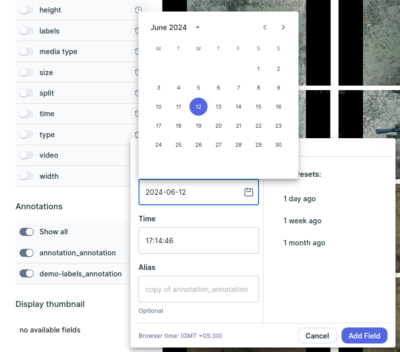
You can also query a condition in a specific time, by selecting the clock icon next to a metadata column, and choosing the date you want to query as of:

Tip

You can also set aliases to semantically indicate meaningful timestamps.

Next steps

Now that you have your dataset ready, move on to visualize it, add annotations, or convert it to a dataloader for training.