Motivation

In the last article, we walked through how to build, train, and evaluate an emotion recognition model.

During the evaluation stage, we found that the model struggled with certain class labels due to low representation in the dataset. The model was also overfitting due to its high complexity, which made it difficult to generalize for new data.

💡 We can solve both issues by training our model on more data.

By enriching our data we can improve the model’s ability to generalize to new data by providing additional unique data samples to train on.

This might seem trivial, but the configuration process requires heavy MLOps lifting. To avoid that, we'll use DagsHub Client, which enables streaming data from multiple sources by adding a few lines of code.

Introduction

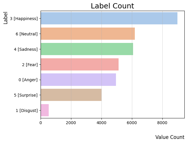
We utilized a VGG19 model pre-trained on the ImageNet dataset for our emotion recognition model. We trained it on the FER Dataset, which has image pixels mapped to 7 possible emotion labels. You can access the class distributions here. Clearly the dataset is imbalanced as label “1” which represents “disgust” only has 547 samples. After running multiple experiments with different sets of hyper parameters we found the best performing model with a training accuracy of 0.72 and a validation accuracy of 0.67. This will serve as our benchmark.

Next Steps

In this article, we will dive into how we can train an emotion recognition model on multiple data sets using the AffectNet dataset and DagsHub Direct Data Access (DDA) for streaming capabilities.

Training the model on different datasets exposes the model to a broader range of variations, enabling it to learn more comprehensive and discriminative feature representations. We will cover how to use transfer learning to train our VGG19 model on both datasets while creating a scalable architecture.

Project Architecture

Let’s take a high-level look at our project architecture.

We host our FER and AffectNet data sets in separate DagsHub repositories versioned with DVC and in a third repository our code and the facial recognition model.

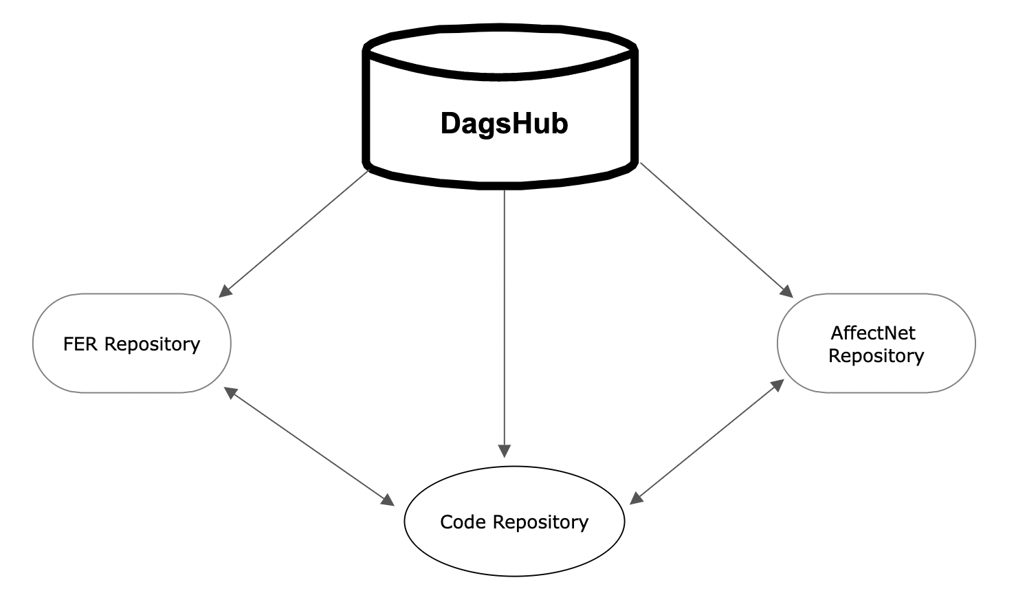
We will create two iterations of training. First, we will stream the data from the FER data repository in one script, train the model, and save the weights. Next, we will load the weights into the same model in another script and stream the data from the AffectNet repository using DDA to train the model on.

Any changes made to the data will only update the data repositories, while changes to the code and model will update the code repository. This helps maintain data integrity, allows for effective collaboration by minimizing conflicts from simultaneous modifications, and enhances scalability which we will touch on later.

Data Repositories

Let’s take a look at the data we are using.

FER dataset

The FER dataset is pre-processed with flattened pixels of 48x48 grayscale images mapped to 7 possible emotion classes. The repository has both the raw and processed data which includes the train and validation files. If you are interested in learning how the raw data was processed, refer to this script.

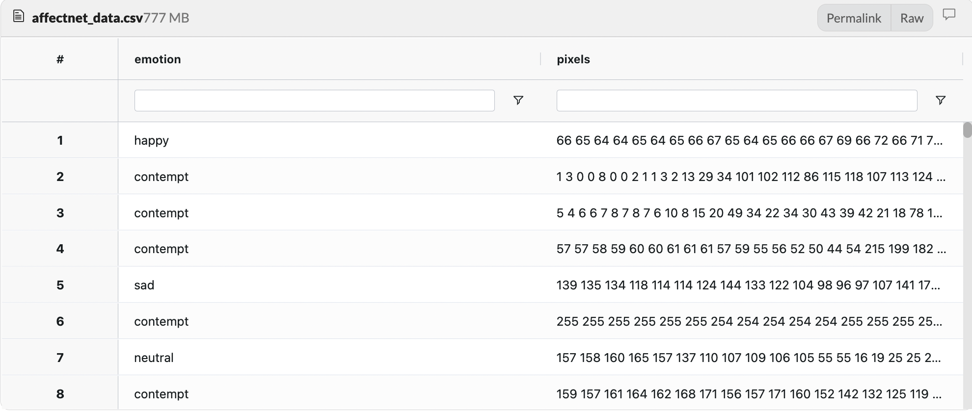
AffectNet dataset

The AffectNet dataset has a set of images stored in labeled folders with a data file of the image paths mapped to its corresponding label. The raw data is compromised of image paths and image labels. Unlike the FER dataset, the AffectNet is much more balanced, which will help the model generalize better during the second training iteration.

{'surprise': 4616, 'happy': 4336, 'anger': 3608, 'disgust': 3472, 'contempt': 3244, 'fear': 3043, 'sad': 2995, 'neutral': 2861}

We also need to standardize the raw data in order to make it compatible with the FER dataset. We will use the following script to access each image path, flatten the images, and store them as a string of separated pixel values, similar to how the FER data file is formatted.

# Create an empty DataFrame to store the image pixels and labels
data = pd.DataFrame(columns=['emotion', 'pixels'])
start_index = 3241
# Iterate over each row in the labels DataFrame
for i in range(start_index, len(df)):
    row = df.iloc[i]
    img_path = join(path, row['pth'])
    img = Image.open(str(img_path)).convert('L')  # Convert image to grayscale
    img_pixels = np.array(img).reshape(-1).astype('int')
    img_pixels_str = ' '.join(map(str, img_pixels))
    emotion = row['label']
    data.loc[i] = [emotion, img_pixels_str]

data.to_csv('data/raw/affectnet_data.csv', index=False)

After standardizing the data and writing it to a csv, we can utilize Direct Data Access to upload the csv file to the remote AffectNet repository.

You will need to pip install dagshub to use DagsHub’s upload API. In addition, you will need to specify the username, repository name, and data paths. Because we are uploading large data files, we will version our data with DVC.

from dagshub.upload import Repo

repo = Repo("GauravMohan1", "Emotion-Data-Repo-Two")
repo.upload(local_path="data/raw/affectnet_data.csv", remote_path="data/raw/affectnet_data.csv", versioning="dvc")

Our AffectNet csv file is now in our remote repository. to go Now we have our two data repositories that we can utilize in our main project repository.

Project Details

The most effective way to train this model on multiple datasets is to use transfer learning, as this will allow for iterative improvements and customizability. Transfer learning from one dataset to another can save time and resources, as the model can benefit from the knowledge acquired on previous tasks.

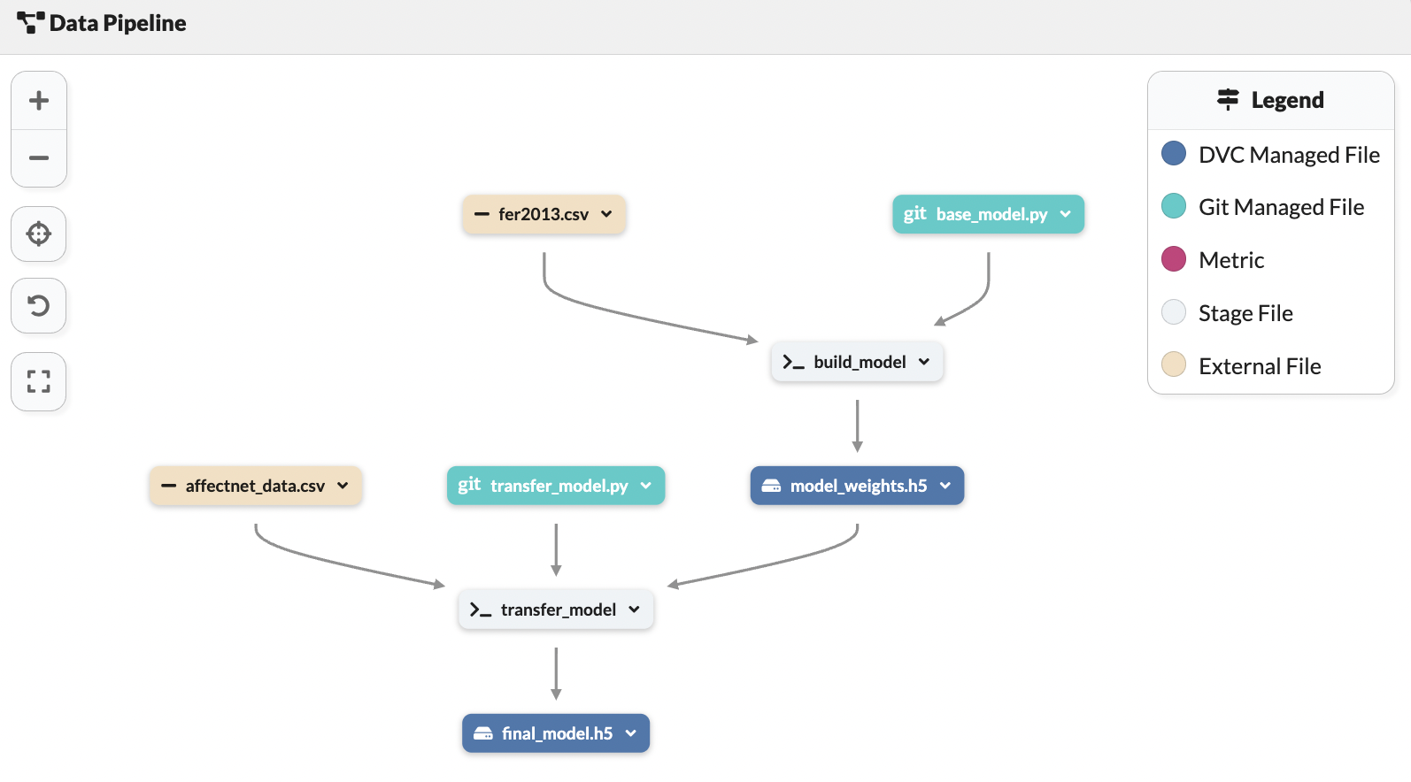
The build model stage will handle the first iteration of training the model. We will train the model on the FER dataset in this stage. We will then save the weights of the model after the training completes.

In the transfer model stage, we will load the model weights to train the model on the AffectNet data. We will evaluate the performance of the model after the second training iteration and output the final model. Use this repository to refer to the code as we dive into it.

Build Model

We will first load the train and validation data from the FER data repository and stream the data using DDA’s python hooks to train our VGG19 model on it. We need to specify the repo_url which will be the link to our DagsHub data repository. We also need the project_root, which is the local path to our cloned data repository that is associated with our remote repository.

import numpy as np
from dagshub.streaming import install_hooks
install_hooks(repo_url="<https://dagshub.com/GauravMohan1/Emotion-Data-Repo>",
            project_root="/Users/gauravmohan/Documents/Emotion-Data-Repo")

import pandas as pd
X_train = np.load('/data/processed/X_train.npy')
y_train = np.load('/data/processed/y_train.npy')
X_valid = np.load('/data/processed/X_valid.npy')
y_valid = np.load('/data/processed/y_valid.npy')

We will need to authorize DagsHub to access the repository data files. We can accomplish this by setting up an env variable “DAGSHUB_USER_TOKEN” with our personal DagsHub token.

Model Structure

Given that we are training a model on two different datasets we can freeze some of the earlier convolution blocks that have more low-level features and train it on the FER dataset. Freezing layers will also reduce the complexity of the model and potentially reduce overfitting. The FER dataset is larger than the AffectNet dataset so it will represent the “source” dataset. The knowledge and learned features from the pre-trained model will then be transferred to a new model, which is trained on a smaller, more specific “target” dataset, which will be the AffectNet dataset. During the second training iteration we will unfreeze an additional block to train the smaller AffectNet dataset on.

The VGG19 model contains 5 convolution blocks that have trainable parameters. For the first training iteration, we will use the 4th and 5th convolution block. These blocks have a lot of trainable parameters that are more high level and can be tuned to classify images on different emotions.

Since we have a large amount of features, we need to apply regularization with larger penalties on earlier blocks.

# code taken from base_model.ipynb 
vgg = VGG19(weights='imagenet', include_top=False, input_shape=(48, 48, 3))

for layer in vgg.layers:
  if layer.name.startswith('block4_conv'):
    layer.trainable = True
    if hasattr(layer, 'kernel_regularizer'):
      print('yes')
      layer.kernel_regularizer = regularizers.l2(0.03)
    else:
      print('added')
      layer.add_weight_regularizer(regularizers.l2(0.03))
  elif layer.name.startswith('block5_conv'):
    layer.trainable = True
    if hasattr(layer, 'kernel_regularizer'):
      print('yes')
      layer.kernel_regularizer = regularizers.l2(0.02)
    else:
      print('added')
      layer.add_weight_regularizer(regularizers.l2(0.02))
  else:
      layer.trainable = False

In addition, we will apply funneling to the model by adding 3 dense layers with iterative drops in unit size to help reduce overfitting, improve the performance on test data, and make the training more efficient. As the layers become progressively smaller, the model becomes more specialized and can learn to better differentiate between classes.

base_model = vgg.layers[-2].output
base_model = GlobalAveragePooling2D()(base_model)
base_model = Dense(512, activation='relu', kernel_regularizer = regularizers.l2(0.01))(base_model)
base_model = Dense(256, activation='relu')(base_model)
base_model = Dense(128, activation='relu')(base_model)

It's important to note that the model architecture will more or less stay the same as we train on different datasets so adding the regularization and funneling in the first training iteration is necessary to handle overfitting and improve model performance in the long run.

We will apply ImageDataGenerator for additional data samples, add early stopping to reduce overfitting, and test different batches sizes and epochs. We won’t go into depth about these techniques as they were covered in the past article.

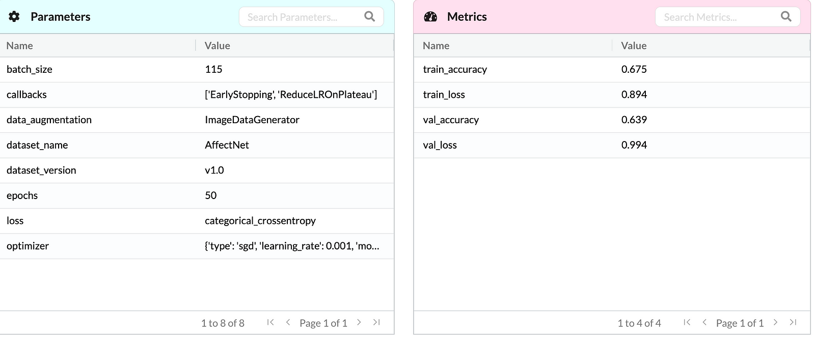
When tracking experiments with MLflow, you will need to specify the tracking uri to store the experiments in DagsHub and the MLflow credentials will need to be exported as environmental variables prior to running experiments. You can find your credentials under the Experiments tab when you click the Remote button in your DagsHub repository. In addition, we will log the dataset used to differentiate which training iteration the experiment is associated to.

import mlflow
mlflow.set_tracking_uri("<https://dagshub.com/GauravMohan1/Dual-Emotion-Recognition.mlflow>")
mlflow.set_experiment("FER")

dataset_name = "FER"
dataset_version = "v1.0"

with mlflow.start_run():

  history = model.fit(train_datagen.flow(X_train, y_train, batch_size=batch_size), 
              validation_data=(X_valid, y_valid), 
              epochs = epochs,
              steps_per_epoch = len(X_train) / batch_size,
              shuffle=True,
              callbacks=[early_stopping, lr_scheduler],
              use_multiprocessing=True,
              class_weight=class_weights_dict)
  
  mlflow.log_param("dataset_name", dataset_name)
  mlflow.log_param("dataset_version", dataset_version)

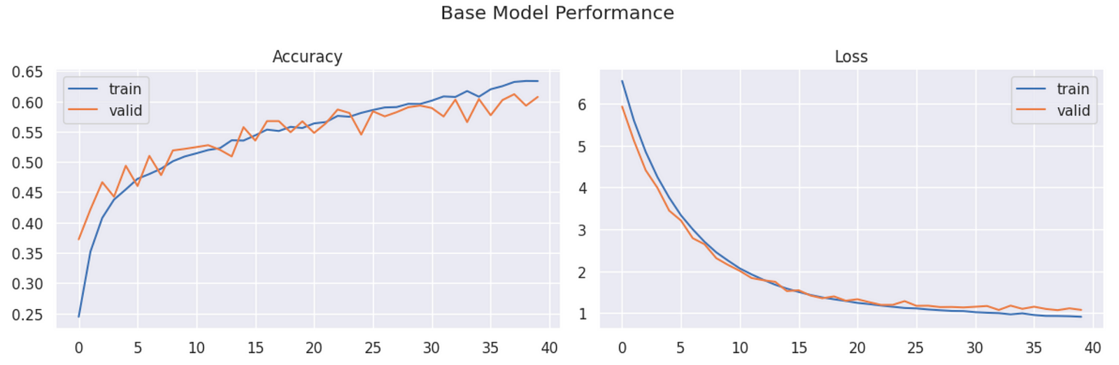
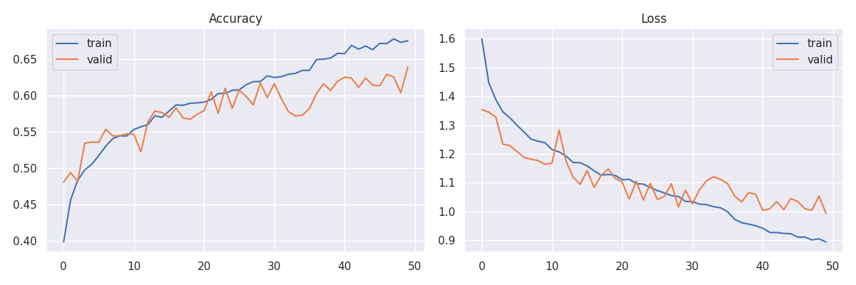
The best experiment yielded a training accuracy of 0.63 and a validation accuracy is 0.61. The model weights are then saved and stored as outputs in the first stage. Notice how the model doesn’t overfit when we freeze some of the layers.

Transfer Model

In the transfer model stage we will load the model weights from the first training iteration and train the model on the AffectNet dataset. However, we first need to preprocess our dataset to match the format of the first data set. The first step is to remove the rows with the label contempt. The AffectNet dataset has 8 labels compared to FER’s 7. The class labels are all similar except for contempt, so we need to mask this label and reset the index.

import numpy as np
from dagshub.streaming import install_hooks
install_hooks()
import pandas as pd

df = pd.read_csv('data/raw/affectnet_data.csv')
#ignore contempt so that we only have 7 of the same classes
df = df[df['emotion'] != 'contempt']
df = df.reset_index(drop=True)  # Reset the index of the DataFrame

The other major change is to down sample the images from a 96x96 inputs into a 48x48 inputs to match the input of the VGG19 model in the first training iteration.

from skimage.transform import resize

#Convert 96x96 to 48x48
pixels = df.pixels.apply(lambda x: np.array(x.split(' ')).reshape(96, 96).astype('float32'))

img_array = []
for i in range(len(pixels)):
    img = pixels[i]
    # Downsample the image by a factor of 2 using averaging
    img = resize(img, output_shape=(48, 48), anti_aliasing=True)
    img_array.append(img)

img_array = np.stack(img_array, axis=0)

After preprocessing the data and splitting it into train, test, and validation datasets it’s time to build the second iteration of the model. The model structure will remain the same, where we unfreeze convolution block 4 and 5 and then add the 3 dense layers. We should utilize the same regularization penalties and unit sizes to make sure the model is the exact same prior to loading the weights to ensure effectiveness. Prior to compiling the model however, we will unfreeze convolution block 3.

for layer in vgg.layers:
    if layer.name.startswith('block3_conv'):
        layer.trainable = True
        if hasattr(layer, 'kernel_regularizer'):
          print('exists')
          layer.kernel_regularizer = regularizers.l2(0.03)
        else:
          print('added')
          layer.add_weight_regularizer(regularizers.l2(0.03))
    else:
        layer.trainable = False

The model now has an additional 2.5 million parameters that it can be trained on. While the majority of the training is done in the first stage, unfreezing a lower level block can help the model learn new patterns and generalize to new data. I also add regularization to the layers to reduce overfitting.

During the first training iteration there were a lot more trainable parameters, so we had to use a low learning rate to adhere to the complexity. For the second training iteration we can use a higher learning rate since we only have 1 convolution block of trainable parameters.

After running numerous experiments the best parameters and model performance are found. The experiment results are shown below.

Evaluation and Next Steps

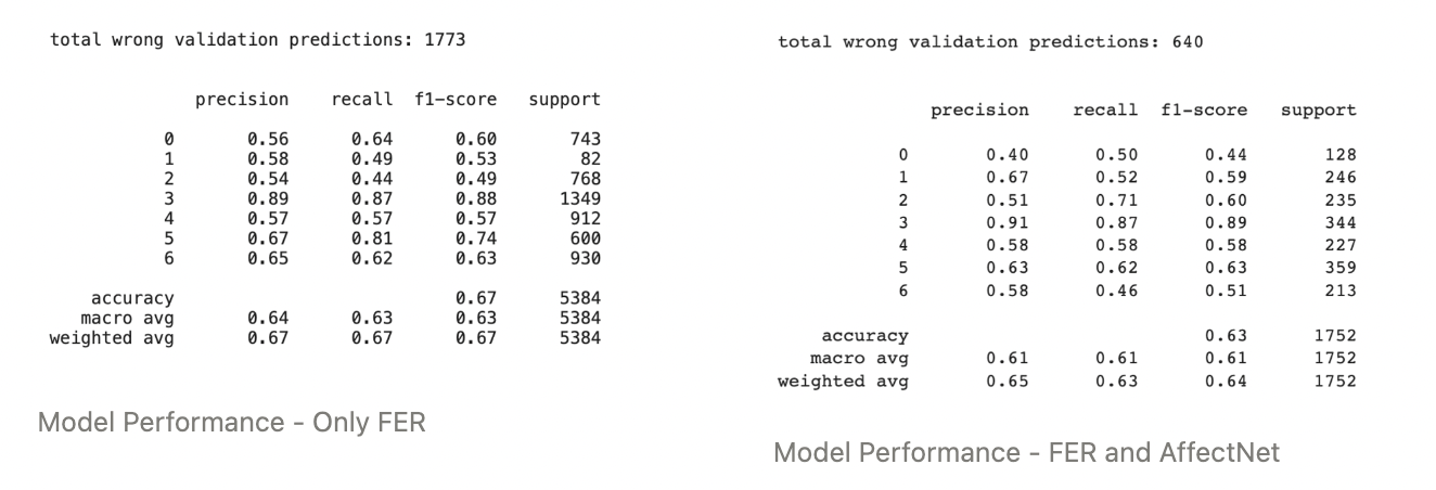
In the test dataset we are using a subset of the AffectNet data. Although we took a stratified split of the train and test data, there seems to be fewer samples of the anger and neutral label in our test data*.* It may make sense to create a combined test dataset with both the FER and AffectNet to balance the samples more. Overall, the model has a much more balanced F1-score across every class label compared to when it is only trained on one dataset. On the left hand side you can see the performance of the model from the previous article. The F1 scores have a much greater variability due to the imbalance of the data and complexity of the model.

Conclusions

Utilizing transfer learning to train the model on multiple datasets gives us  a scalable architecture that allows us have control over how we train the model on each dataset. This in turn allows us to to train the model on more datasets if we need to. Additional data repositories can be initialized and streamed using DDA. The more datasets we train the model on the better it will be at generalizing to new data.

One thing to note is that in this tutorial we decided to keep the standardize notebook separate from the pipeline as it is directly affecting a singular data repository. However, it may make sense to incorporate the standardizing script as part of the preprocess stage prior to the transfer model stage.

Congratulations! Through this series of posts, you’ve learned a lot about training models on different datasets, streaming data with DagsHub Client, and using transfer learning. You rock!