Train An Emotion Recognition Model Using Open Source MLOps Tools
- Gaurav Mohan
- 11 min read
- 3 years ago
I am a Data Science professional and enjoy exploring and blogging about new AI/ML mechanisms through applied use cases.

Introduction
This tutorial takes you on a journey to construct an emotion recognition model using the renowned VGG model and the comprehensive FER dataset. We delve into the fundamental principles of emotion recognition, explore the rationale behind VGG, and dive into the FER dataset. We then go over all the project components and processes, from data preparation, model training, and experiment tracking to model evaluation, to equip you with the skills to construct your own emotion recognition model.
Refer to this repository as we walk through the project.
Project Overview
For this project, we’re going to be utilizing a VGG19 model pre-trained on ImageNet. VGG models have achieved strong performance on the ImageNet benchmark, which indicates their ability to generalize well to different visual recognition tasks. It is very accurate in image recognition and has a deep network and with small 3x3 convolutional filters. While other models like ResNet allow for even deeper networks and performs inference faster, VGG generalizes better which is important in facial recognition tasks.
Let’s take a moment to break down the project architecture shown above before we dive into the code.
What is the FER dataset?
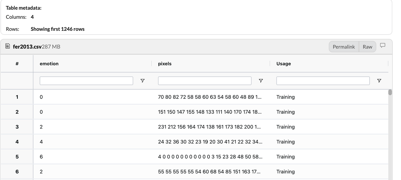
FER, Facial Expression Recognition, is an open-source dataset released in 2013. It was introduced in a paper titled "Challenges in Representation Learning: A Report on Three Machine Learning Contests" by Pierre-Luc Carrier and Aaron Courville. It holds cropped facial images of size 48x48 pixels, represented in a flattened array of 2304 pixels.
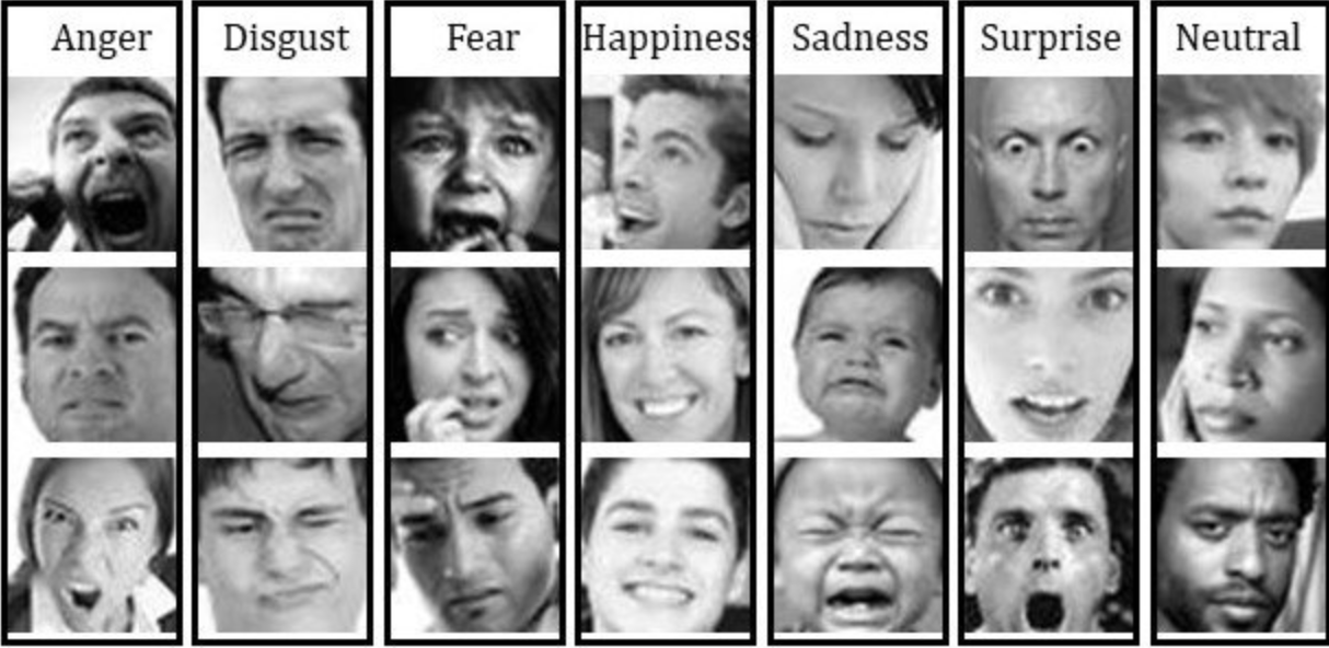
Each image is labeled with a representative emotion using the following mapping: {0:'anger', 1:'disgust', 2:'fear', 3:'happiness', 4: 'sadness', 5: 'surprise', 6: 'neutral'}
Data pipeline overviews
The pipeline in this project is managed by DVC and has three stages:
- Process data: extracts the image features, encodes the labels, splits the dataset to train, and test, and saves them to file.
- Model: utilizes the training data to train a model and tune the hyper-parameters.
- Analyze: evaluates the model’s performance using the validation data.
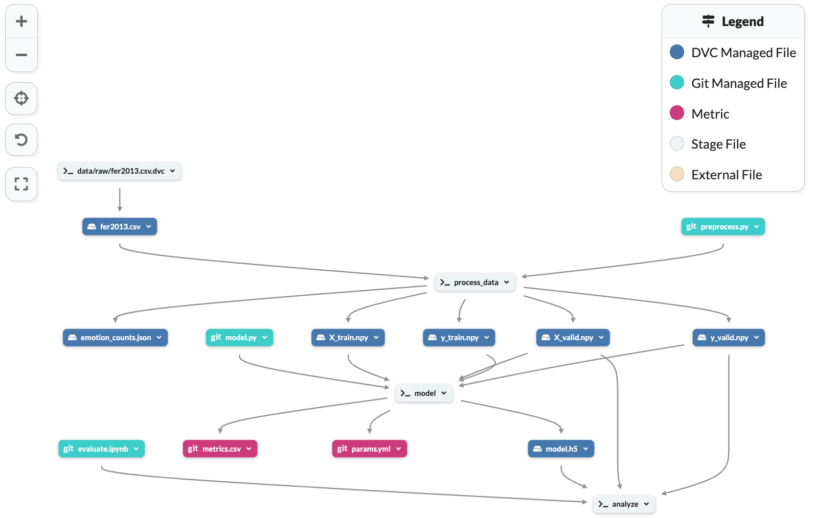
The full pipeline is shown here.
Data Processing
The preprocess script covers all the necessary steps to get our data ready for training. It has five main steps:
- Converted the string pixels into (48, 48, 3) image arrays.
- Encoded the labels
- Split the data into train and validation using stratified split
- Saved the train/validation as numpy data files
- Pushed the data files to our remote DagsHub repository
The data is first reshaped into a 48x48 numpy 2D array in order to make it compatible with the VGG model. The arrays are then iteratively converted from grayscale to RGB. By converting grayscale images to RGB, we make it compatible with the pre-trained VGG model and effectively replicate the grayscale intensity values across all three channels, allowing the model to benefit from color-based features during training. The corresponding labels are then encoded using the following code:
from keras.utils import to_categorical
labels = df['emotion'].values
encoded_labels = to_categorical(labels, num_classes=7)
Finally, the data is split into a train and validation set using a stratified split.
Model Development
Now that we have our training and validation data, it is time to build the model, train it, and run experiments to improve performance using the model script. The following image shows a standard VGG19 model and one shown after re-orchestrating the last block of the model.
Something cool I discovered on DagsHub is that it visualizes the model’s architecture using Nitron! You can check it out here.
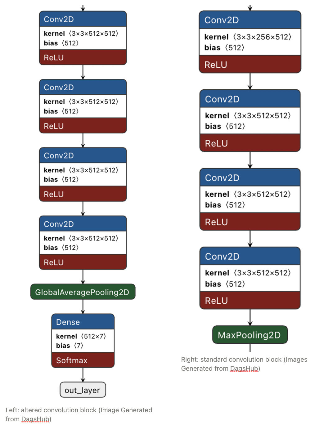
In order to preserve the weights of the model prior to training on a new dataset, we replace the last convolution block with the output layer for the FER dataset, replace the MaxPooling2D with a GlobalAveragePooling2D, and add a final dense layer for the model output.
base_model = tf.keras.applications.VGG19(weights='imagenet', include_top=False, input_shape=(48, 48, 3))

# Add dense layers
x = base_model.layers[-2].output
x = GlobalAveragePooling2D()(x)

# Add final classification layer
output_layer = Dense(num_classes, activation='softmax')(x)

# Create model
model = Model(inputs=base_model.input, outputs=output_layer)
A GlobalAveragePooling2D layer reduces the computation time by computing the average of each feature map, which forces the network to learn features that are globally relevant to the task resulting in a one-dimensional vector with a smaller number of values. While this is the general architecture of the model, it isn’t ready for deployment.
Data Augmentation
In terms of data augmentation, in the prior stage, I stored the counts of each class label within the dataset. As you can see this is an imbalanced dataset; there are much more data points for happiness, neutrality, and sadness compared to disgust and surprise.
{"3": 8989, "6": 6198, "4": 6077, "2": 5121, "0": 4953, "5": 4002, "1": 547}

emotion labels → {0:'anger', 1:'disgust', 2:'fear', 3:'happiness', 4: 'sadness', 5: 'surprise', 6: 'neutral'}
There are two ways we can handle the imbalanced dataset. The first way is to actually generate more data using ImageDataGenerator. This is commonly used in deep learning tasks to generate more training samples through random rotations, translations, shearing, zooming, flipping, and other image modifiers. Applying this technique will help the model generalize better and improve the accuracy on the test set given that this model is skewed to certain labels. The implementation is shown below. The data generator is fitted on the training set and incorporated into the model as it is training.
train_datagen = ImageDataGenerator(rotation_range=20,
width_shift_range=0.20,
height_shift_range=0.20,
shear_range=0.15,
zoom_range=0.15,
horizontal_flip=True,
fill_mode='nearest')

train_datagen.fit(X_train)
The second method to handle an imbalanced dataset is to pass in the class weights while the model is training. The resulting weights can be used to balance the loss function during training. Class weights are automatically adjusted to the frequencies of the input data as: n_samples / (n_classes * np.bincount(y))
class_weights = compute_class_weight(
                                        class_weight = "balanced",
                                        classes = np.unique(y_train.argmax(axis=1)),
                                        y = y_train.argmax(axis=1)
                                    )
class_weights_dict = dict(enumerate(class_weights))

## Now train the model
history = model.fit(train_datagen.flow(X_train,
                                       y_train,
                                       batch_size = batch_size),
                                       validation_data = (X_valid, y_valid),
                                       steps_per_epoch = steps_per_epoch,
                                       epochs = epochs,
                                       callbacks = callbacks,
                                       use_multiprocessing = True,
                                       class_weight=class_weights_dict)
The class_weights_dict is passed along with the train_datagen to generate random batches of data and balance the loss function.
The callbacks, early stopping and learning rate scheduler, also handle overfitting by reducing the learning rate if the loss doesn’t reduce over the epochs or stopping the training completely.
lr_scheduler = ReduceLROnPlateau(monitor = 'val_accuracy',
                              factor = 0.25,
                              patience = 8,
                              min_lr = 1e-6,
                              verbose = 1)

early_stopping = EarlyStopping(monitor = 'val_accuracy',
                            min_delta = 0.00005,
                            patience = 12,
                            verbose = 1,
                            restore_best_weights = True)
The patience parameter states how many epochs of continuous performance decline need to occur before the callback is applied to the training process.
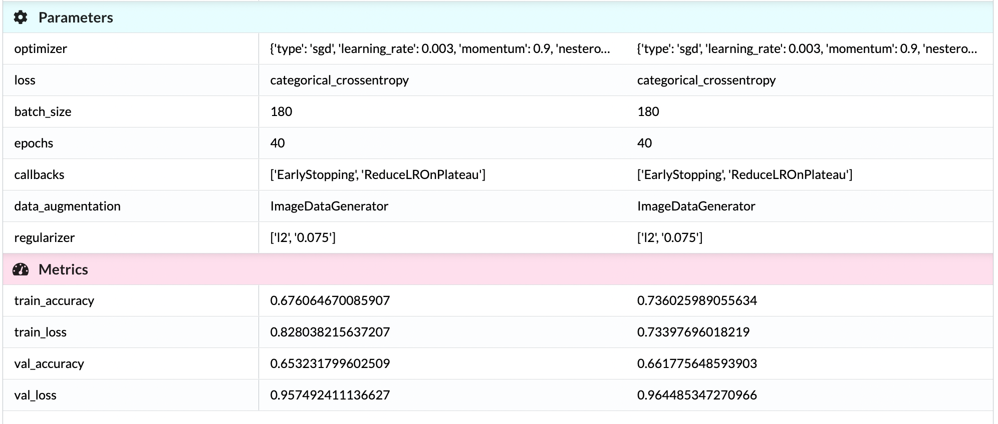
We can compare two experiments run with matching parameters. The only change between the models is that the class weights are incorporated during the training. As you can see the model performs slightly better with this addition. The train_loss is significantly reduced and the validation accuracy also improves slightly.
Hyper Parameter Search
The next step in tuning the model is to find the best-fitting hyper parameters. One way to accomplish this is to use a Keras tuner. The Keras tuner is a built-in module that can be applied to Keras models by searching for a specific set of hyper parameters that are provided.
I created two different experiments. The first one is focused on testing different sets of optimizers, learning rates, batch sizes, and epochs. We will use the tune_model.ipynb to run these experiments.
The parameters are passed as hp objects. They are given a min and max value and a step value to provide a range of values that can be tested. In the first iteration of search, we want to test different combinations of batch size, epochs, and learning rate.
from kerastuner.engine.hyperparameters import HyperParameters
from kerastuner.tuners import RandomSearch

hp = HyperParameters()
batch_size = hp.Int('batch_size', min_value=16, max_value=256, step=16)
epochs = hp.Int('epochs', min_value=10, max_value=50, step=10)
The hp objects are passed into the build model function and a different set of values are tested on each trial. The number of trials is set as max trials. Depending on the number of hyper parameters, the step size, and overall range, it may make sense to increase or decrease the number of trials so that the tuner is able to effectively search enough combinations of these parameters. The goal is to maximize the validation accuracy as shown below.
tuner = RandomSearch(build_model, objective='val_accuracy',
										 max_trials=10,
										 hyperparameters=hp)

tuner.search(train_datagen.flow(X_train, y_train, batch_size=batch_size),
             validation_data=(X_valid, y_valid),
             epochs=epochs,
             callbacks=[early_stopping, lr_scheduler, mlflow_callback],
             use_multiprocessing=True)
MLFlow Callback
One callback that is shown that we have not discussed yet is the mlflow_callback. The callback tracks the changes in model accuracy at the end of each epoch and logs it to DagsHub as an experiment. In order to incorporate it within the keras tuner, I created an MLflow class to track the change in validation accuracy after each epoch in a trial.
class MlflowCallback(Callback):
    def __init__(self, run_name):
        self.run_name = run_name

    def on_train_begin(self, logs=None):
        mlflow.set_tracking_uri("<https://dagshub.com/GauravMohan1/Emotion-Classification.mlflow>")
        mlflow.start_run(run_name=self.run_name)

    def on_trial_end(self, trial, logs={}):
        hp = trial.hyperparameters.values
        for key, value in hp.items():
            mlflow.log_param(key, value)

        mlflow.log_param('epochs', 32)
        mlflow.log_param('batch_size', 212)
        mlflow.log_param('learning_rate', 0.003)

        mlflow.log_metric("val_accuracy", logs["val_accuracy"])
        mlflow.log_metric("train_accuracy", logs["train_accuracy"])
        mlflow.log_metric("val_loss", logs["val_loss"])
        mlflow.log_metric("train_loss", logs["val_loss"])


    def on_train_end(self, logs=None):
        mlflow.end_run()

mlflow_callback = MlflowCallback('layers add')
The mlflow callback sets the tracking uri at the start when the keras tuner starts its search. You will need to configure mlflow with your own credentials. You must export the tracking username and password as environment variables in your project shell prior to setting the tracking uri as shown below.
export MLFLOW_TRACKING_USERNAME=<your username>
export MLFLOW_TRACKING_PASSWORD=<your password/token>
When the trial is completed the metrics and hyper parameters that are logged will be stored within the experiments tab in the DagsHub repository. A plot is also generated to show the following change in accuracy over each epoch.
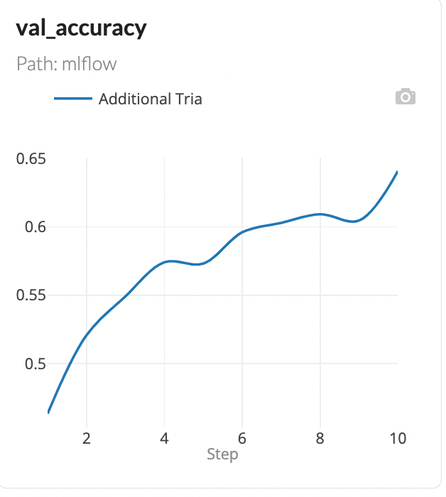
I found that the SGD optimizer worked the best along with a low learning rate, large batch size, and an epoch range from 30 to 40. Here is the experiment that yielded the best results for these set of parameters..
The next set of parameters searched is additional dense layers, the number of units within these layers, and the regularization penalty. The best parameters from the first search is passed into these next trials.
# Define the hyperparameter search space
# Now I want to test if adding additional layers and adding regularization will help improve overfitting or improve accuracy
hp = HyperParameters()
num_dense_layers = hp.Int('num_dense_layers', min_value=1, max_value=3)
num_units = hp.Int('num_units', min_value=64, max_value=512, step=32)
reg_strength = hp.Float('reg_strength', min_value=0.001, max_value= 0.1, step=0.004)

tuner.search(train_datagen.flow(X_train, y_train, batch_size=212),
             validation_data=(X_valid, y_valid),
             epochs = 32,
             steps_per_epoch = len(X_train) / 212,
             callbacks=[early_stopping, lr_scheduler, mlflow_callback],
             use_multiprocessing=True)

best_hp = tuner.get_best_hyperparameters()[0]
mlflow.log(best_hp.values)
The reason we add additional layers and apply regularization is to see if a higher learning rate and epoch count can be effective. The downside of doing this is that it can cause overfitting which did occur in some experiments. However, adding additional dense layers along with L2 regularization can mitigate the overfitting.
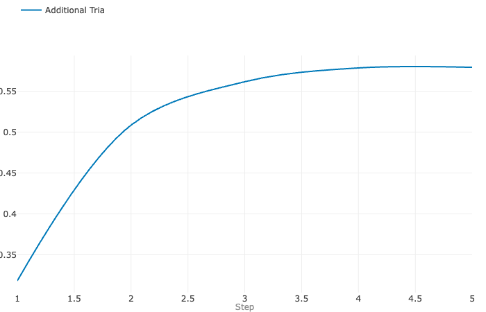
The model did not seem to respond well to added layers and plateaued in accuracy over the course of training.
Experiment Tracking
Once you have found a set of parameters that perform well, you no longer need to use the keras tuner. We can once again train the model and log the parameters using MLFlow. After setting the tracking uri and starting the run, we will build and train the model as shown before. Now we can define all the parameters and log the results at the end of the run.
mlflow.set_tracking_uri("<https://dagshub.com/GauravMohan1/Emotion-Classification.mlflow>")
with mlflow.start_run():
    # batch size of 32 performs the best.
    model = build_model(num_classes)

    history = train(model, X_train, y_train, X_valid, y_valid)
    metrics = {"train_accuracy": history.history['accuracy'][-1], "val_accuracy": history.history['val_accuracy'][-1],
               "train_loss": history.history['loss'][-1], "val_loss": history.history['val_loss'][-1]}

    params = {"optimizer": {'type': 'sgd', 'learning_rate': 0.0092, 'momentum': 0.90, 'nesterov': True}, "loss": 'categorical_crossentropy', 'batch_size': 96,
              'epochs': 24, 'callbacks': ['EarlyStopping', 'ReduceLROnPlateau'], 'data_augmentation': 'ImageDataGenerator'}

    mlflow.log_metrics(metrics)
    mlflow.log_params(params)
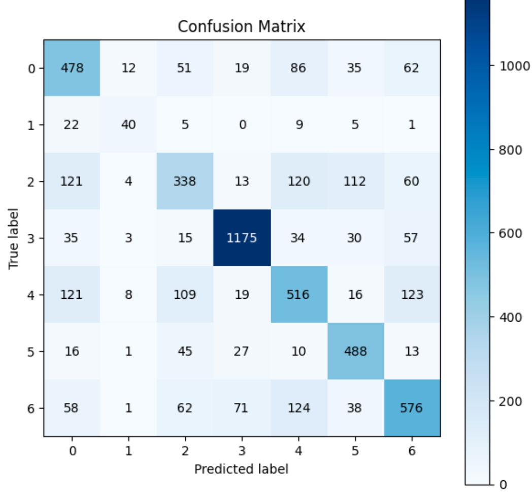
Model Evaluation
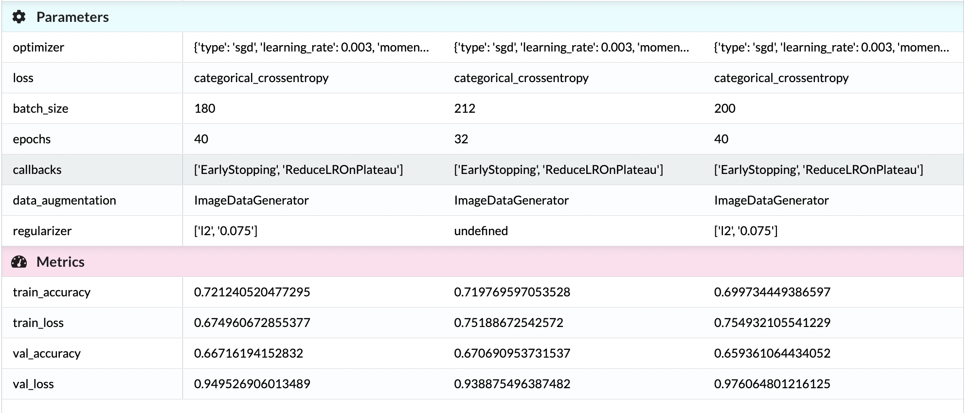
After running multiple experiments, I compared the top 3 performing ones. I wanted to choose a model that maximizes validation accuracy while minimizing the loss. I also compared the training accuracy and loss to make sure the model wasn’t overfitting too much. The second model performs the best. I saved this model in my repository.
The last step in the model process is to evaluate the performance of the model. We utilize papermill to execute the evaluation notebook in a separate eval script so it can be handled by the DVC pipeline.
Let’s look at the results of the model’s performance on the validation dataset.
| precision | recall | f1-score | support | |
|---|---|---|---|---|
| anger | 0.56 | 0.64 | 0.60 | 743 |
| disgust | 0.58 | 0.49 | 0.53 | 82 |
| fear | 0.54 | 0.44 | 0.49 | 768 |
| happiness | 0.89 | 0.87 | 0.88 | 1349 |
| sadness | 0.58 | 0.57 | 0.57 | 912 |
| surprise | 0.67 | 0.81 | 0.74 | 600 |
| neutral | 0.65 | 0.62 | 0.63 | 930 |
| accuracy | 0.67 | 5384 | ||
| macro avg | 0.64 | 0.63 | 0.63 | 5384 |
| weighted avg | 0.67 | 0.67 | 0.67 | 5384 |
Total Wrong Validation Predictions: 1773
Insights and Conclusions
Given that we are using an imbalanced data set, the model is struggling to accurately predict the disgust, fear, and sadness labels due to the lack of samples provided in the test. The lack of training samples for specific class labels is a major problem in many multi-class classifiers. In addition, the model is overfitting even with the callbacks and regularization added. This may be because we are using every trainable parameter in the VGG model to tune to the dataset, instead of potentially freezing some layers. Due to the complexity and number of parameters in the model it may struggle to generalize to new data.
It may be useful to train this model on different datasets to improve its ability to generalize against new data, reduce bias on certain class labels, and improve the overall performance of the model.
We can accomplish this by hosting different datasets in their own repository and utilizing DagsHub Client to stream the data and train the model on multiple datasets in an efficient way using a concept called transfer learning. Stay tuned for the next article to see how this is accomplished.
Additional Resources
If you are interested in streaming the data directly from the remote repository, you can utilize the main branch of the project. The main branch utilizes DagsHub’s Direct Data Access, which is an API that connects to the remote repository in DagsHub to stream data. The scripts execute the same logic, however, it does not utilize the DVC pipeline to store files as dependencies and receive file objects. Instead, it utilizes Python Hooks to stream datasets that are already in the remote repository. Refer to the repository’s README to see how you can modify your project to stream the data directly from the remote repository.
If you have any questions, feel free to reach out. You can join our Discord, where we’ve built a vibrant, helpful and friendly community.