Tutorial: Build an Active Learning Pipeline using Data Engine

An end-to-end active learning pipeline is something many struggle with. Even large companies with experienced data science teams run into issues.

The main issue tends to be the tooling. Most of the time, tooling for an active learning pipeline needs to be either custom written, or cobbled together from several different open source tools.

With the release of Data Engine, DagsHub has made it easier to create an active learning pipeline. In this tutorial, we will learn about Data Engine and see how we can use it to create an active learning pipeline for an image segmentation model using the COCO 1K.

Easy peasy, lemon squeezy.

Setup

Start by forking the COCO_1K repo.

Once that's done, we can start writing some Python. We can do this in a Jupyter or Colab Notebook, or in a script.

We begin by setting up some constants for the project:

# Environment Variables
DAGSHUB_USER= "<username>"
DAGSHUB_REPO_OWNER = DAGSHUB_USER
DAGSHUB_REPO="COCO_1K"
DAGSHUB_FULL_REPO=DAGSHUB_REPO_OWNER + "/" + DAGSHUB_REPO
DATASOURCE_NAME = "COCO_1K_Demo"
MLFLOW_PROJECT = "Default"

Make sure to put your DagsHub username in the appropriate places.

Next, we import all the modules we need:

import yaml
import torch
import mlflow
import ultralytics

from utils.config import Config
from utils.dagshub_yolo_cb import custom_callbacks_fn
from utils.data import DataFunctions

import dagshub
from dagshub.data_engine import datasources, datasets

Of the first set of modules, two are somewhat interesting. mlflow is used to log training parameters, metrics and artifacts to the DagsHub repo's MLflow server. ultralytics is used to train a YOLOv8 image segmentation model.

The next set of imports are helper classes and functions from the repo's utils submodule. Feel free to get familiar with them.

The final imports are the DagsHub client library and the Data Engine.

To finish setting up, we add the following code:

classes = Config.classes
dataset_func = DataFunctions(dataset_dir="data/", classes=classes, label_type='segmentation')

Both Config and DataFunctions were imported from the repo’s utils folder.

dataset_func will allow us to create metadata and YAML files more easily for our flow. The metadata will be used by the Data Engine ad the YAML files are needed to train YOLOv8.

That’s all for the initial setup we need to do!

Upload Data

The repo we forked already contains training and validation images in the data folder. However, if you're creating a project from scratch, you'll need to upload your data to the repo.

For completion sake, here's how we can do that:

dagshub.upload_files(repo=DAGSHUB_FULL_REPO, local_path="data", remote_path="data", commit_message="Upload COCO_1K Dataset")

This uses the DagsHub client library to upload files from our local path to our repo and version them by dvc. No need to mess with command-line DVC!

Create a datasource

Once we have data available in our repo, we can use Data Engine to create a datasource out of it.

To do so, add the following code:

# Create the datasource
ds = datasources.create_from_repo(DAGSHUB_FULL_REPO, DATASOURCE_NAME, "data/images")

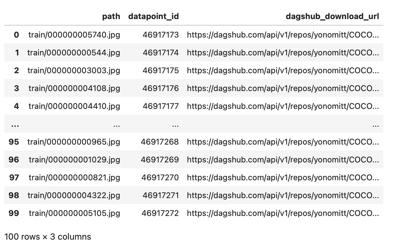
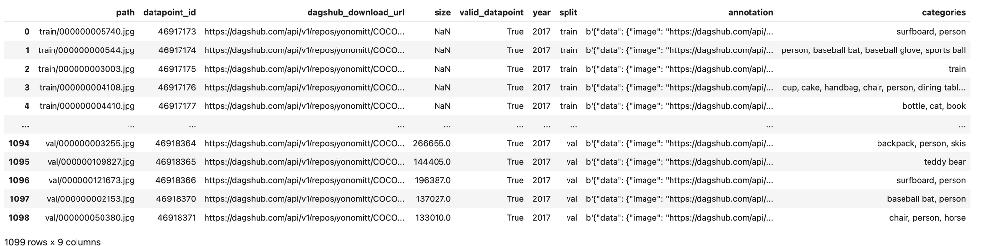
# Display a table of the first entries in the datasource using a Pandas Dataframe
ds.head().dataframe

When run in a Jupyter notebook, our Dataframe head should look something like:

Get a datasource

If we already have a datasource, we can get it by running:

ds = datasources.get_datasource(DAGSHUB_FULL_REPO, DATASOURCE_NAME)

Sometimes, we also want to slice a datasource by filtering based on path. For instance, let's say we already have a repo with labeled data in it. During the active learning cycle, we collect and add new data to the datasource, but we upload to a new_data folder. We could then filter the datasource to remove this new, unlabeled data by running:

ds = ~(ds['path'].contains("new_data"))

This will filter out any images which have new_data in their path. There are other ways to do this in our projects. For instance, we can add metadata (see next section) to indicate whether the image has been processed or not.

Enrich the metadata

Data Engine allows us to enrich our datasource with metadata. This can be anything from annotations to timestamps to information we might want to filter datasources on.

We're going to use a helper method to add annotations and some other metadata to our datasource:

# Get all samples in data source
md_query = ds.all()
# Convert the query into a dataframe
md = md_query.dataframe

# Add metadata to each sample in the dataframe
enriched_md = md.apply(lambda x: dataset_func.create_metadata(x), axis=1)

If we were to look at enriched_md now, we would see the following new information we added:

• valid_datapoint - boolean indicating whether the datapoint has been processed
• year - COCO dataset year
• split - whether the images belongs to the training, validation, or test set
• annotation - Label Studio-formatted annotations
• categories - the set of categories for the annotations present in the images

Finally, we need to upload the metadata to DagsHub Data Engine and make it accessible outside our local machine and to all team members:

dagshub.common.config.dataengine_metadata_upload_batch_size = 50
ds.upload_metadata_from_dataframe(enriched_md, path_column="path")

Visualize the data

After adding metadata, we can visualize the data along with its metadata using the integration with Voxel's FiftyOne.

First, we clear any existing data from the visualizations:

import fiftyone
try:
    fiftyone.delete_dataset(DATASOURCE_NAME)
except:
    print("No dataset to delete")

Then, we download the annotation blob field and cache it locally:

ds.all().get_blob_fields("annotation")

Finally, we start FiftyOne:

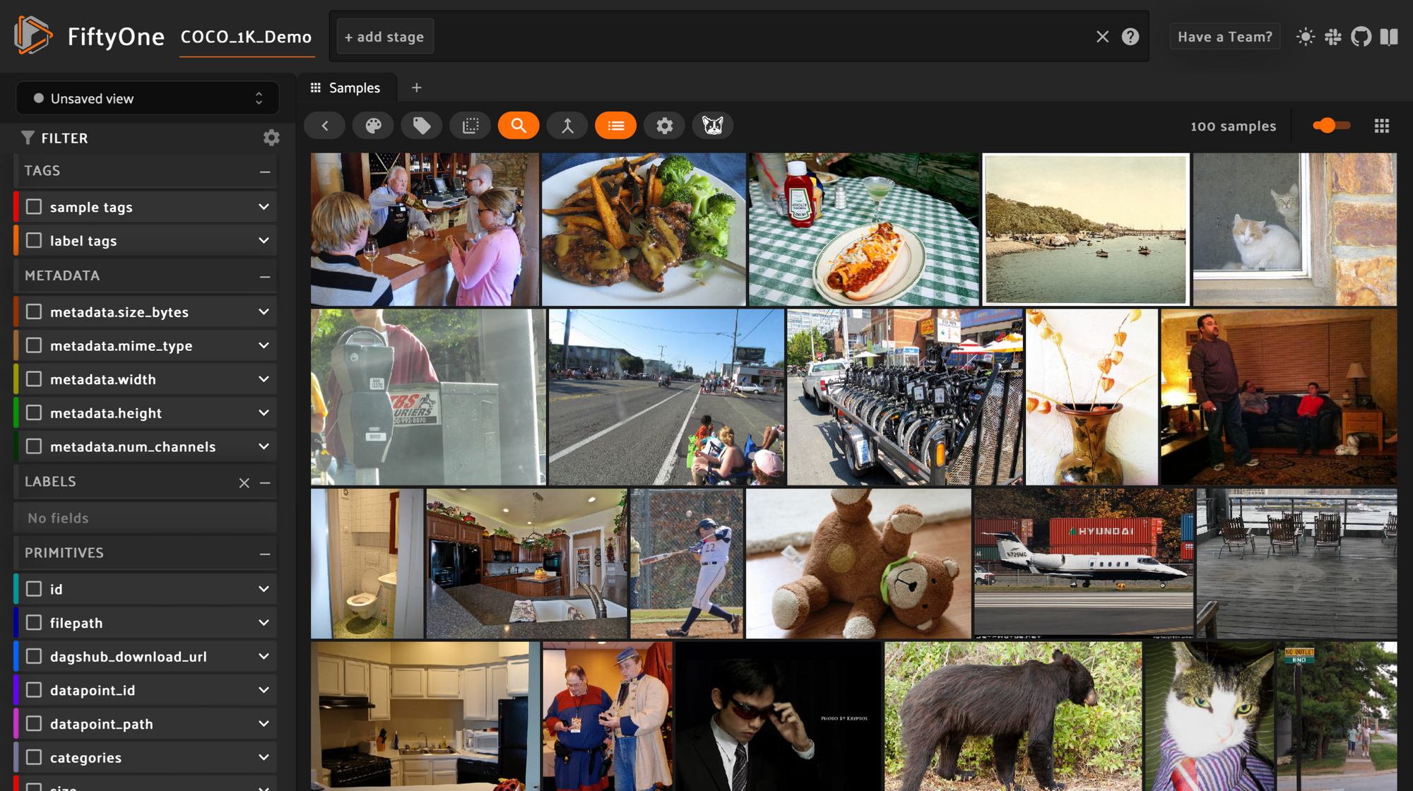
ds.head().visualize()

When we run this last line in a Jupyter Notebook, FiftyOne should display in the output. It will be completely interactive.

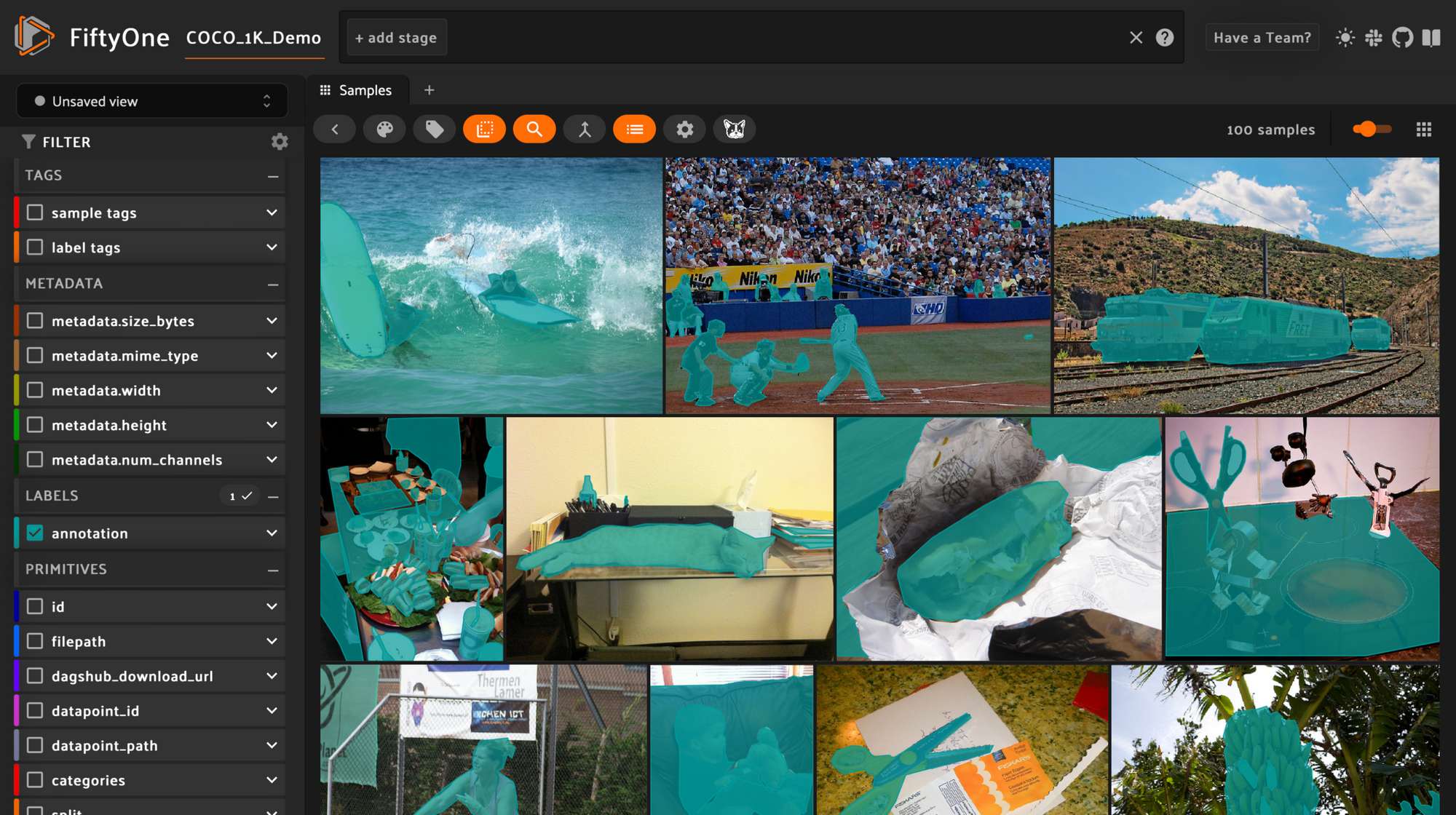
This visualization step is important for data scientists to create an intuition for the data they're working with. It allows them to also make informed hypotheses, they can then test.

Train an initial model

It's now time to train our first model. This model will eventually be used in our active learning pipeline to help automatically annotate new data we collect in the future.

As previously mentioned, we'll be training Ultralytic's YOLOv8 image segmentation model. The repo for YOLOv8 makes it super easy to start training a new model.

First, we need to create a YOL0v8-compatible dataset from our Data Engine datasource:

dataset_func.create_yolo_v8_dataset_yaml(ds)
ultralytics.utils.callbacks.add_integration_callbacks = custom_callbacks_fn

The create_yolo_v8_dataset_yaml() helper function creates the YAML file YOLOv8 uses to determine where the training, validation, and test data are located. Additionally, we also monkey-patch the add_integration_callbacks()function in order to add a custom callback for MLflow.

We then setup our DagsHub client, load a pre-trained YOLOv8 image segmentation model, and start training:

# Setup DagsHub with the local machine
dagshub.init(repo_name=DAGSHUB_REPO, repo_owner=DAGSHUB_USER)

# Load a pretrained model (recommended for training)
model = ultralytics.YOLO('yolov8n-seg.pt', task='segment')  

with mlflow.start_run():

    # Train the model
    model.train(data='custom_coco.yaml', epochs=1, imgsz=640, device='mps', project=MLFLOW_PROJECT)

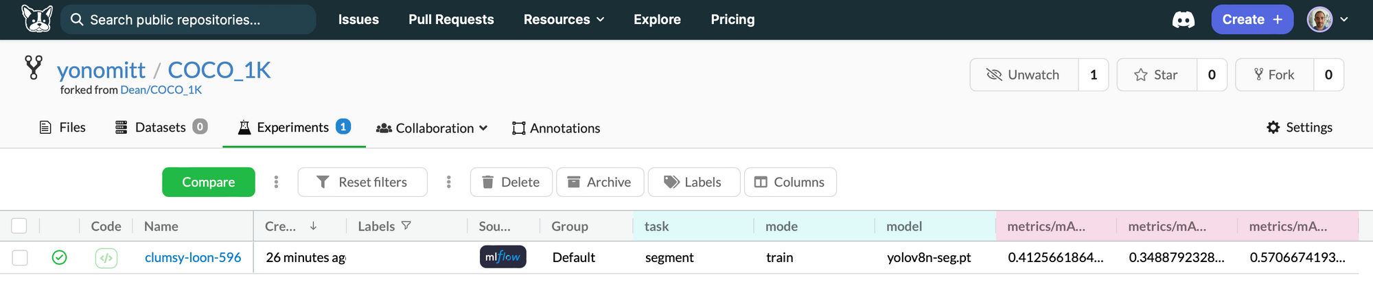
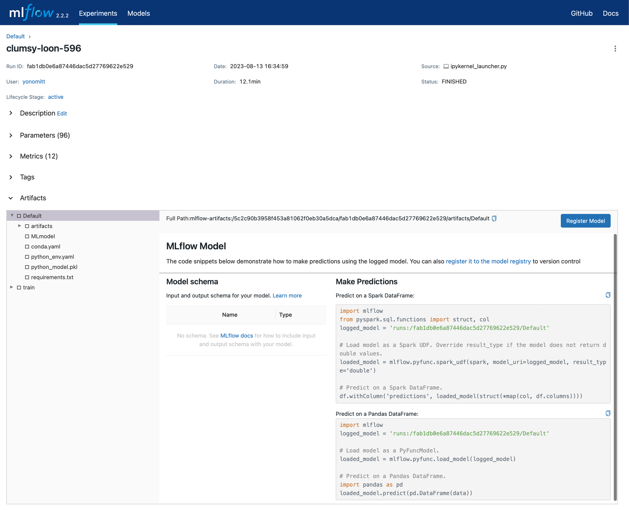
Upon completion, the training parameters and metrics, as well as the trained model will be logged to the MLflow repo associated with our repo.

Add more data

Once we have a model, the next step is to collect more data, so we can improve our model.

In the interest of simplifying this tutorial, the repo already contains a data/images/train/new_data folder with images that were not used in training above. This means the next two code blocks do not need to be run. They are only presented for informational purposes.

After we collect new data, we can run a command like this to copy it to the training folder in the repo:

mkdir data/images/train/new_data && cp -r new_data/* data/images/train/new_data

We would then need to upload the files to our repo using the DagsHub client:

import dagshub
dagshub.upload_files(repo=DAGSHUB_FULL_REPO, local_path="data/images/train/new_data", remote_path="data/images/train/new_data", commit_message="Add new data")

After this, we need to rescan the datasource on DagsHub, under the Datasets tab (see the sync button below)

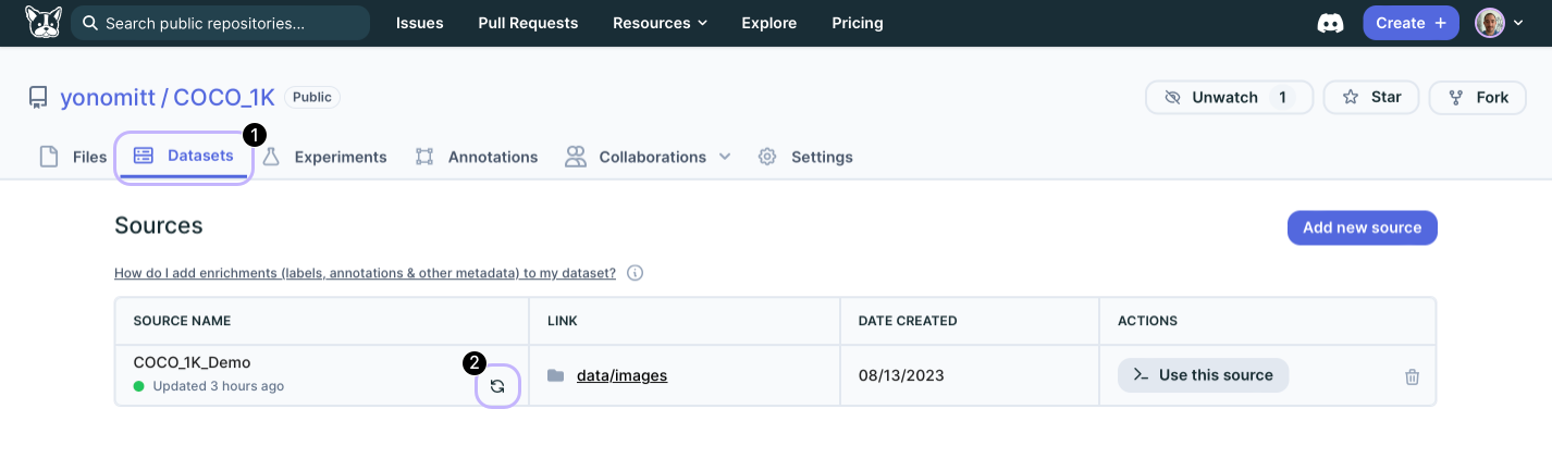
Once we've rescanned the datasource, we have access to the new data in our pipeline.

First, we get our datasource, the same way we did earlier:

from dagshub.data_engine import datasources
ds = datasources.get_datasource(DAGSHUB_FULL_REPO, DATASOURCE_NAME)

Next, we want to filter out all data, which already contains enriched metadata. We do this by checking whether the metadata contains a valid_datapoint field. Previously, the create_metadata() method we used set this field to Truewhen creating the metadata. This is a handy way to determine which data has metadata and which doesn't:

new_data_q = (ds["valid_datapoint"].is_null())
new_data = new_data_q.all()
new_md = new_data.dataframe

Then, we add metadata to this new data using the same function and upload the metadata to the datasource:

enriched_new_md = new_md.apply(lambda x: dataset_func.create_metadata(x), axis=1)

dagshub.common.config.dataengine_metadata_upload_batch_size = 50
ds.upload_metadata_from_dataframe(enriched_new_md, path_column="path")

As mentioned earlier, we want to visualize our new data to spot-check and ensure we understand it:

new_data.visualize()

Auto-annotate data

In order to auto-annotate our data using our trained model, we need to run a Label Studio ML Backend. This is a webserver that has a specific set of endpoints, which Label Studio can talk to. For more in-depth information, checkout Automate the Labeling Process with Label Studio.

To start the ML backend, run the following command in a terminal from the repo's root.

make create_ls_backend

Once we have our Label Studio ML Backend running, we’re ready to setup a Label Studio project for our repo.

Run:

new_data.annotate()

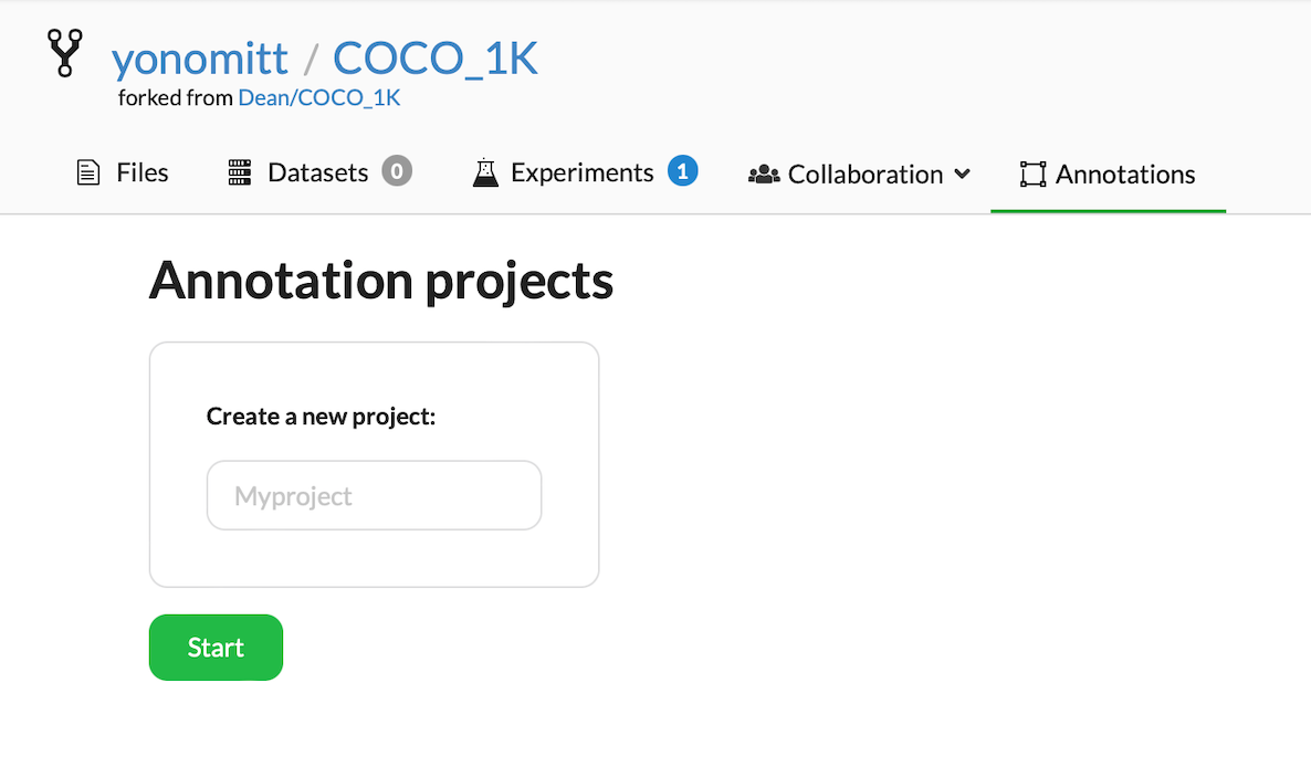
This opens DagsHub’s integration of Label Studio in a browser. Using Label Studio, we need to perform the following steps:

1. Give Label Studio a project name, like New Labels or First Iteration and click Start. Label Studio will then load all the tasks based on the new data to be labeled as part of the project.

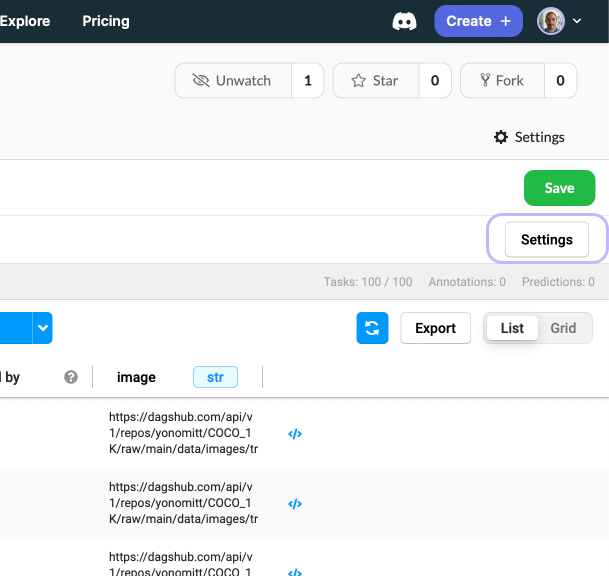
2. Click the Settings button to enter the settings menu

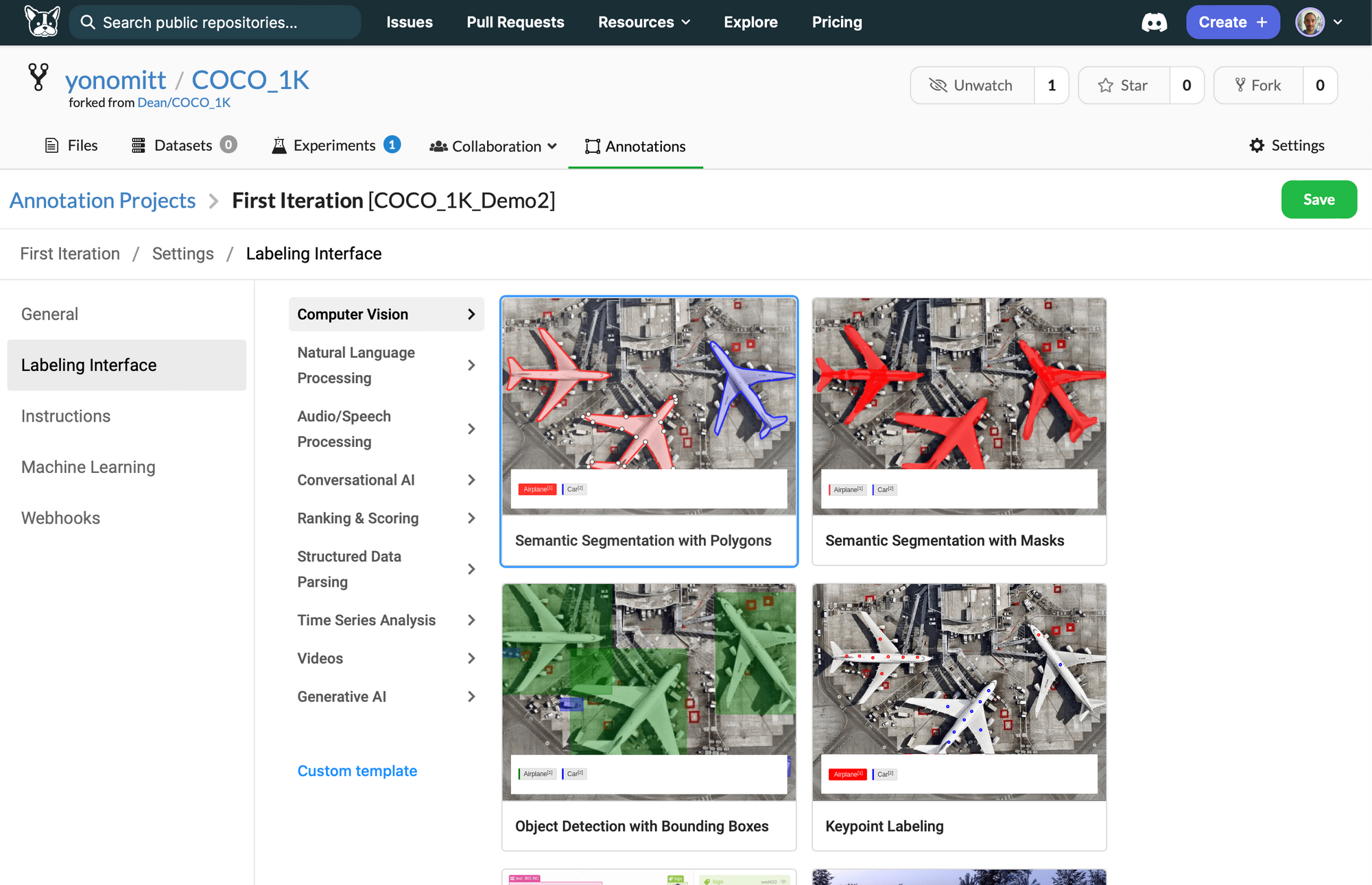
3. Click on the Labeling Interface tab and then the Browse Templates button

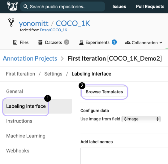
4. Select the Semantic Segmentation with Polygons template

5. Add the label names

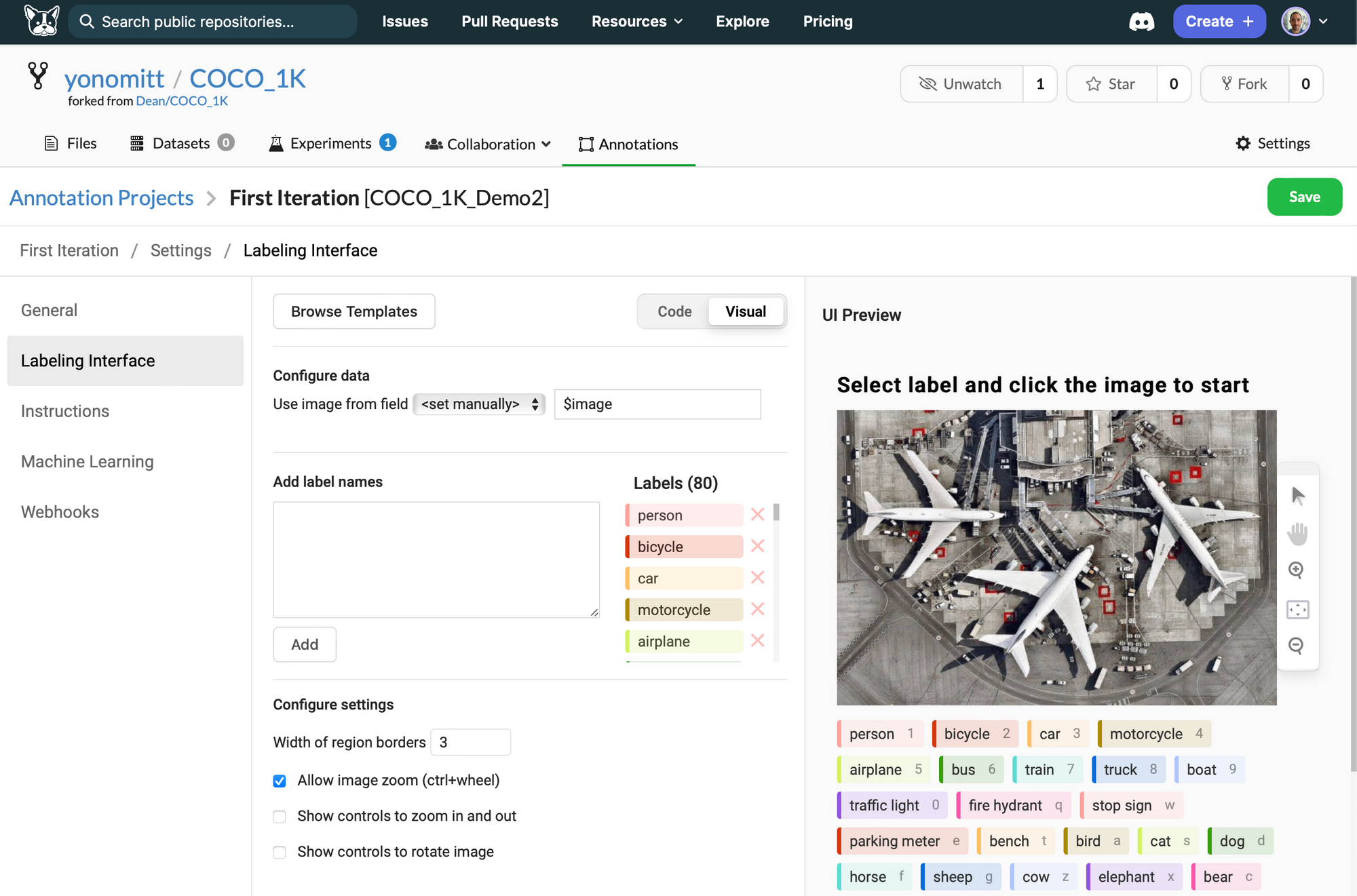
To simplify this, you can run a for loop to print out all class names and then copy and paste the output into the Add label names text field

for label in Config.classes:
    print(label)

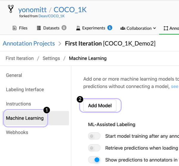
6. Click on the Machine Learning tab and then the Add Model button

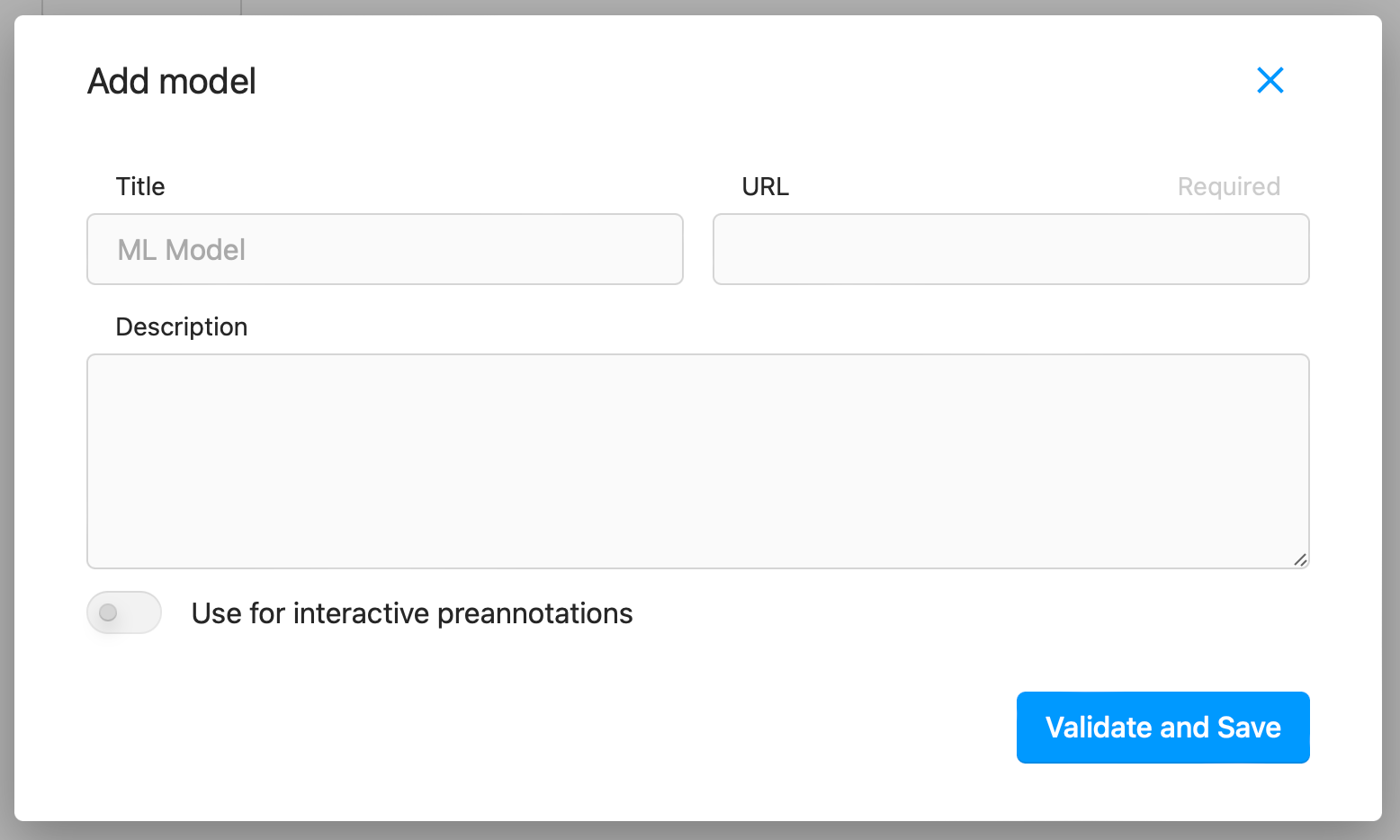
7. Add the URL ngrok provides for your machine and click Validate and Save

Once we’ve connected it, we can send tasks to our backend, which will run inference on the data and create predictions from them.

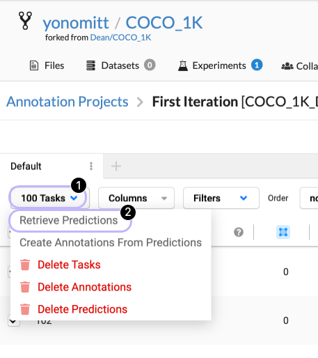
8. Go back to the task list and select all tasks by clicking the checkbox next to ID

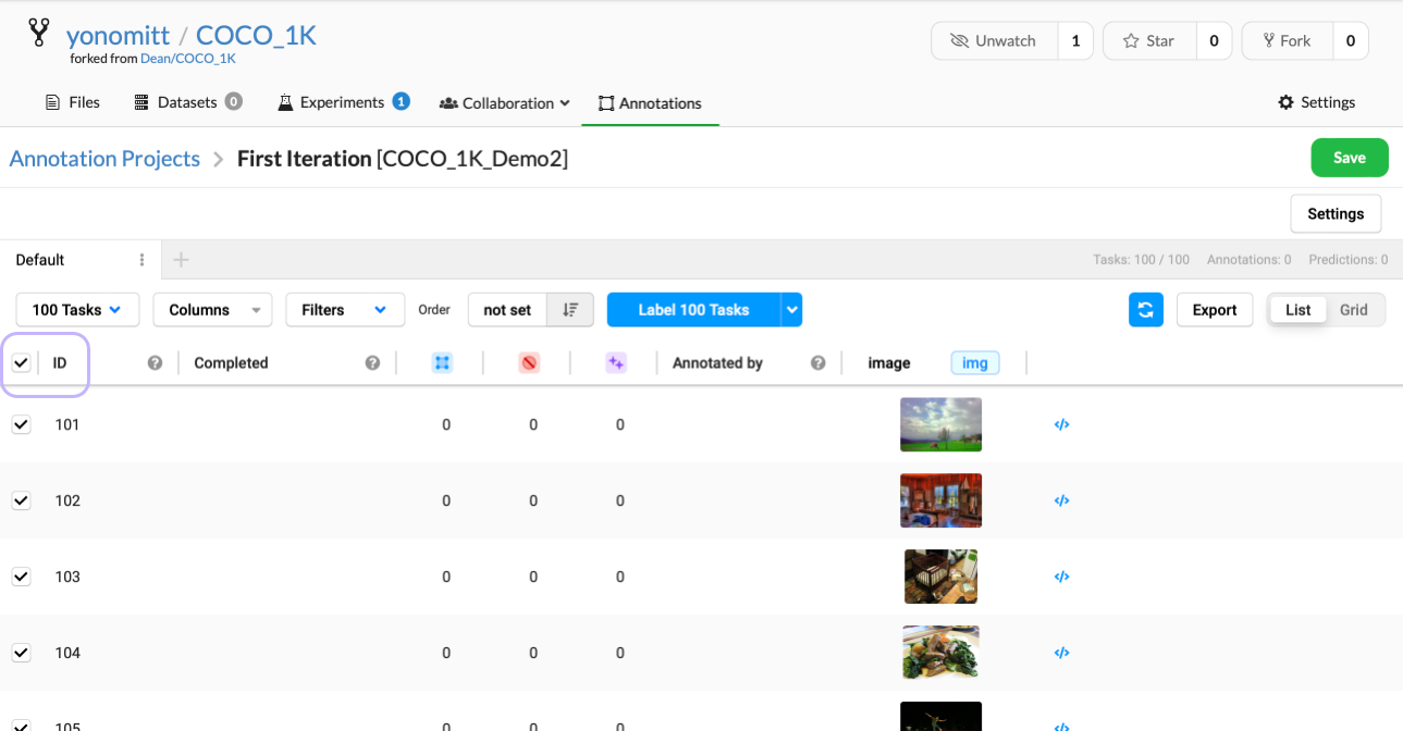
9. Click the Tasks dropdown menu and select Retrieve Predictions

After all the tasks have been run, we need to convert the predictions to annotations. For that, we return to our notebook.

First, we use the Label Studio SDK to create a client:

from label_studio_sdk import Client
ls = Client(url=f'https://{DAGSHUB_USER}:{dagshub.auth.get_token()}@dagshub.com/{DAGSHUB_REPO_OWNER}/{DAGSHUB_REPO}/annotations/de', api_key=dagshub.auth.get_token())

Then we use the client to find the project ID for the project we just created in Label Studio via the browser:

proj_name = "<Project name we gave to Label Studio>"
ls_id = -1

for proj in ls.list_projects():
    if proj.params['title'] == proj_name:
        ls_id = proj.params['id']
        break

if ls_id < 0:
    print("No project found")

Finally, we use the project to convert all predictions into annotations, assuming they’re all correct:

project = ls.get_project(ls_id)

project.create_annotations_from_predictions()

Train a better model

After using our backend to create annotations for our new data, it's time to train a new and, hopefully, better model.

Most of this code should look familiar. First, we get our datasource:

from dagshub.data_engine import datasources
ds = datasources.get_datasource(DAGSHUB_FULL_REPO, DATASOURCE_NAME)

To ensure our new data was properly annotated, we filter our datasource and visualize the new data:

new_data_q = (ds["path"].contains("new_data"))
new_data = new_data_q.all()
new_md = new_data.dataframe

new_data.visualize()

Next, we set up our dataset using our entire datasource (not just the new data). We also, once again, monkey-patch the YOLOv8 training callbacks:

dataset_func.create_yolo_v8_dataset_yaml(ds)
ultralytics.utils.callbacks.add_integration_callbacks = custom_callbacks_fn

Finally, we kick off the training once again, to close our active learning loop:

dagshub.init(repo_name=DAGSHUB_REPO, repo_owner=DAGSHUB_USER)

# Load a model
model = YOLO('yolov8n-seg.pt', task='segment')  # load a pretrained model (recommended for training)

with mlflow.start_run():

    # Train the model
    model.train(data='custom_coco.yaml', epochs=1, imgsz=640, device='mps', project=MLFLOW_PROJECT)

This will, once again, log all parameters, metrics and the trained model to our MLflow server on DagsHub.

Conclusion

And that's it. This example is possibly the easiest way to set up an active learning pipeline. Almost the entire flow, excluding the Label Studio ML Backend and refreshing the datasource on DagsHub, can be run directly from a Jupyter Notebook!

Try it out for your project and let us know what you think.

Join our Discord Community and let us know. We’d love to hear about your experience.