Implementing an LSTM Architecture to build “Next Word Prediction”
- Yichen Zhao
- 6 min read
- 3 years ago
Graduate Student in MSDS program at University of San Francisco, Data Science Intern at Dagshub

Introduction
Natural Language Processing (NLP) is a significant part of artificial Intelligence that is heavily based on text data. One of the fundamental tasks in NLP is Next Word Prediction, which is to predict the next few words that people most likely anticipate as they type along. We understand that writing blocks of texts and framing a big paragraph are sometimes time-consuming so this project aims to assist message conveyance by having users select a proposed word as opposed to composing it.
We build this language model using LSTM architecture. If you are not familiar with LSTM or RNN, please check out the blog Complete Guide to RNN, LSTM and Bidirectional LSTM. This blog will walk you through how to build a next word prediction model by implementing LSTM architecture step by step.
You can find the project with the data, code, experiments and pipeline on in the DagsHub repository.
Data Preprocessing
The raw dataset we collected for this project is the popular 20 Newsgroups data set, which is a collection of approximately 20,000 newsgroup documents, partitioned (nearly) evenly across 20 different newsgroups. The training and test sets are naturally split when we obtained the dataset.
The first stage is data pre-processing. We need to organize the unstructured text data into a tabular format that most machine learning models can take in.
During this stage, we:
- Tokenize the text
- Filter out non-English words
- Remove words shorter than 3 characters
- Ignore all stop words
# convert all English characters to lower case
text = text.lower()

# keep only English characters
tokenizer = RegexpTokenizer(r'[a-zA-Z]+')
tokens = tokenizer.tokenize(text)

# remove words that have less than 3 letters
tokens = [w for w in tokens if len(w) > 2]

# remove English stop words
tokens = [word for word in tokens if word not in ENGLISH_STOP_WORDS]
The full code can be found here.
After tokenization, we would like to reformat the tokens into a tabular form. To do that, we iterate through every token. For each token, we assign the token at current position as target, and its previous tokens of fixed length as context. In this project, the context window is one-sided and the window size is set to 5, meaning that for every token we take 5 tokens to its left as the context. The window size is one of the hyperparameters that you could try different values with.
Here we provide a toy example of context-target splitting just to make sure that you follow along. If we define the context window size to be 3, using the text “Apple is something that competitors simply cannot reproduce.”, we are able to reorganize this unstructured text into a tabular form:
| context word 1 | context word 2 | context word 3 | target |
|---|---|---|---|
| apple | is | something | that |
| is | something | that | competitors |
| something | that | competitors | simply |
| that | competitors | simply | cannot |
| competitors | simply | cannot | reproduce |
We apply this reformatting technique to both training and test sets and create a tabular training set and a tabular test set.
Word Embedding
The next step is word embedding. Even after the data pre-processing stage converts the unstructured text data to a tabular form, the data itself is still text. However, most machine learning models take in numeric values as inputs and output numeric values. Therefore some sort of word embedding is a must for training a NLP model.
In this project, we take advantage of a pre-trained word embedding model provided by the SpaCy library. This language model converts each English word into a vector of 96 entries.
Check out the code snippet below and full code here that performs the word embedding task described above.
nlp = spacy.load('en_core_web_sm')
for i in tqdm(range(len(context_train))):
    each_words = context_train[i]
    for j, each_word in enumerate(each_words):
				# nlp(each_word) embeds each_word to a 96-vector
        embedded_context_train[i, j, :] = nlp(each_word).vector
    embedded_target_train[i, :] = nlp(target_train[i]).vector
The similarity in meaning of two words is represented by the Euclidean distance between the two corresponding embedded vectors. Through this embedding process the input dimension of each context-target pair becomes 96 x 5.
For the sake of training efficiency, we randomly picked 20,000 context-target pairs from the tabular training set for training, and 2000 context-target pairs from the tabular test set for model evaluation. The reduced train size (20000) and reduced test size (2000) are also user-defined and can vary upon your preference.
Model Training
After getting our dataset ready, we initialize the model training process. We first construct the model using the idea of LSTM: one unidirectional LSTM layer followed by a fully connected layer:
class NWP_LSTM(nn.Module):
    ...
    def forward(self, x):
        ...
        # LSTM layer
        out, _ = self.lstm(x, (h0, c0))
        out = out[:, -1, :]
        # fully connected layer
        out = self.fc(out)
        return out
Since the model is evaluated by the similarity between predicted and actual word vectors, we use negative cosine similarity as the loss function. Additionally we use an Adam optimizer for the model training process. Other model-related hyperparameters that are logged throughout the experiments are listed below:
# loss function and optimizer
criterion = nn.CosineEmbeddingLoss()
optimizer = torch.optim.Adam(model.parameters(), lr=learning_rate)
# these can be tuned
batch_size = 40
hidden_size = 256
num_layers = 2
num_epochs = 50
learning_rate = 0.001
# these are fixed values (related to word embedding method)
input_size = 96
word_vector_size = 96
The hyperparameters “batch_size”, “hidden_size”, “num_layers”, “num_epochs”, “learning_rate” are logged by MLflow so that we are able to keep track of experiment results for different values of these hyperparameters. All we need to do is to add the following block of code to the model training script:
# log hyperparameters
mlflow.start_run()
mlflow.log_params({'model_class': 'unidirectional LSTM',
                  'model': model.parameters(),
                  'optimizer': 'adam',
                  'criterion': 'cosine embedding',
                  'epochs': num_epochs,
                  'batch size': batch_size,
                  'learning rate': learning_rate,
                  'hidden layer size': hidden_size,
                  'number of LSTM layers': num_layers,
                  'context window size': CONTEXT_WINDOW})
mlflow.end_run()
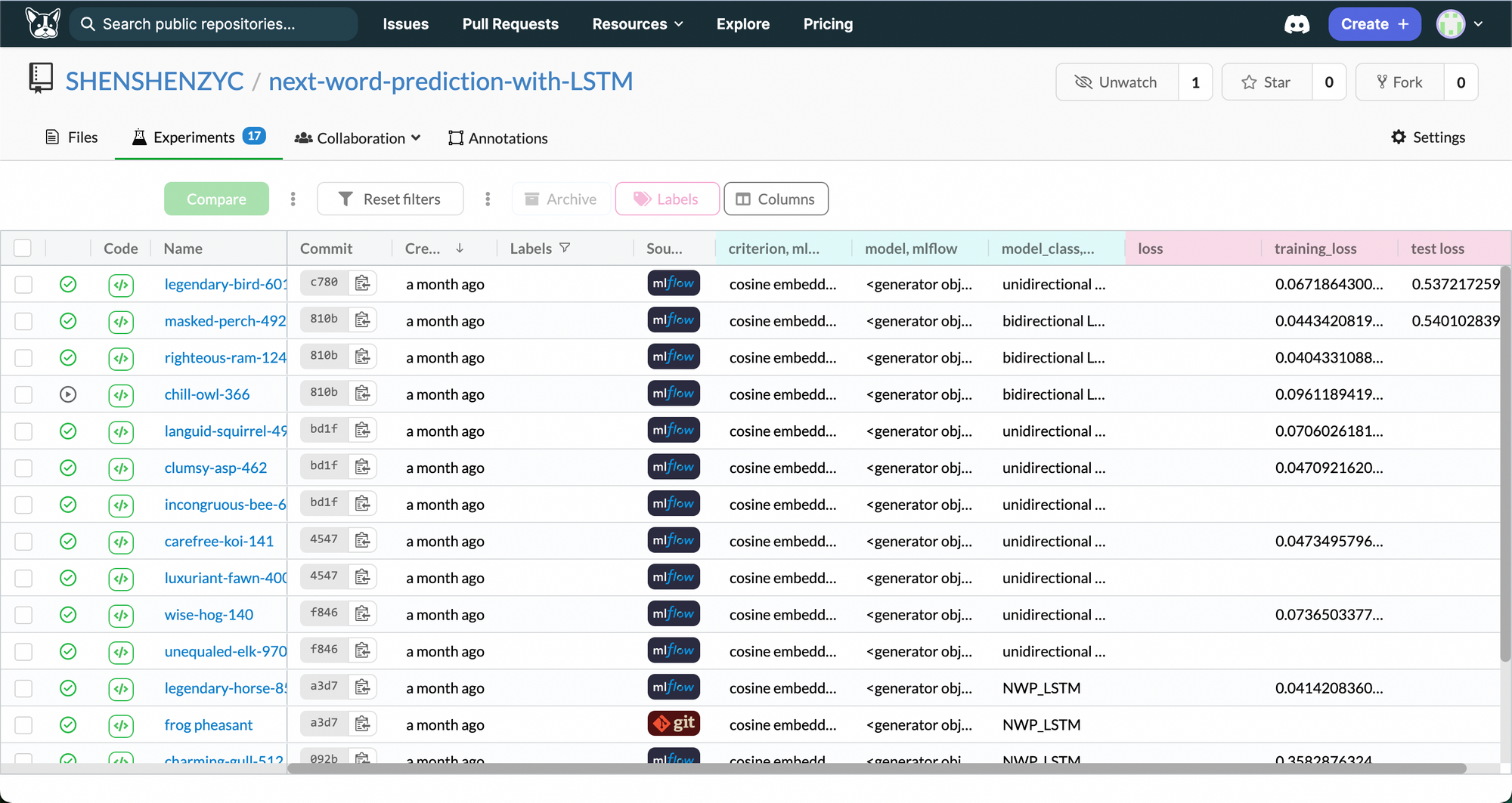
Each experiment will be recorded under the “Experiment” tab of your Dagshub repository. There you are able to go through the list of experiments and locate the model with best performance after you try out different hyperparameter values. The following screenshot from my repository shows you what to expect under the “Experiment” tab.
The following code snippet shows the basic structure of a training loop:
for epoch in range(num_epochs):
    for i, (contexts, targets) in enumerate(train_loader):
        # Forward pass
        preds = model(contexts)
        loss = criterion(preds, targets, torch.tensor([1] * batch_size))

        # Backward and optimize
        loss.backward()
        optimizer.step()
        optimizer.zero_grad()
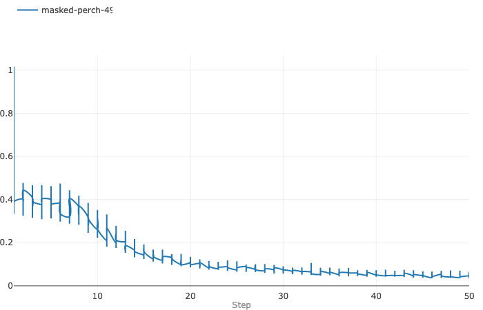
As the training loop runs through the 50 epochs, we would like to visualize the trend of training loss as the number of epochs increases. Here is when MLflow live-logging feature comes in handy. MLflow metric logging function can record the loss value of each epoch and integrate all losses to create a loss vs. epochs plot to visualize the trend of loss, like the one shown below that I download from one of the experiments:
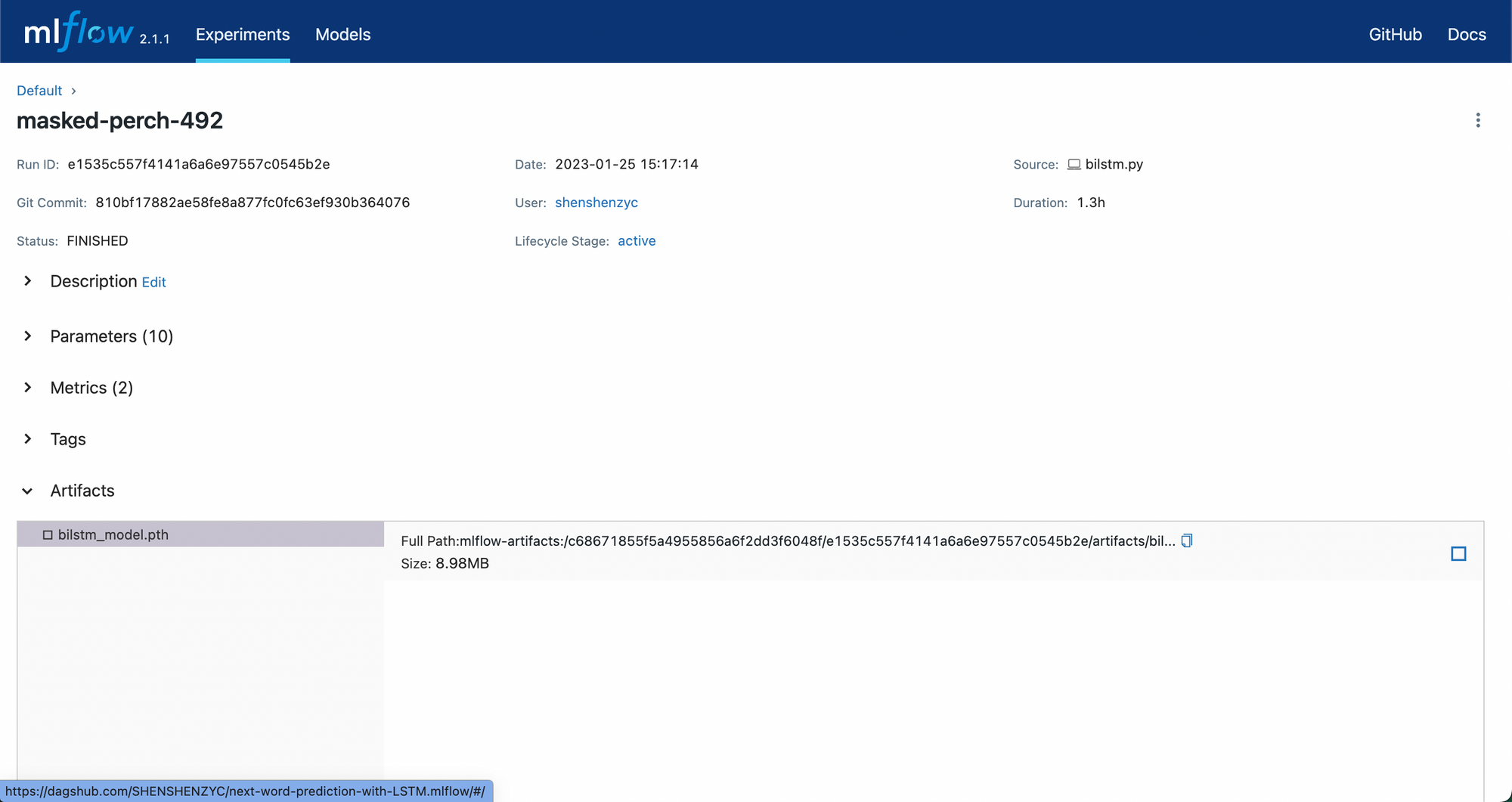
As the model is done training, we evaluate the model performance on the separate test set and record its metric on test set using MLflow. We also log the model artifact using the MLflow artifact logging function after saving the model in the repository. The logged model artifact will be stored in the MLflow server on DagsHub and is available for future access. The screenshot below shows how it looks in the Dagshub MLflow UI for the logged model artifact from the same experiment where the above training loss curve belongs to:
Now we have trained a language model that predicts the next word as people type, and this concludes this project.
Feel welcome to check out python script for more details on how MLflow logging works in practice, and the Experiments tab under the Dagshub repo to see how MLflow integrates with Dagshub platform and what are actually logged for each experiment throughout this project. Also check out the Compare feature supported by Dagshub platform that allows us to parallel the logged trend of training loss (plots) and other logged features of different experiments.