Data-Driven AI in Manufacturing: Casting Defect Identification using Active Learning

As we stand on the brink of the Fourth Industrial Revolution, the way businesses operate has fundamentally changed. Over the next few years, companies using AI technology will grow more rapidly. AI-based industrial automation can help improve product quality and design, save labor costs, shorten manufacturing cycles, and track equipment health in real time.

With the availability of state-of-the-art AI algorithms on open-source repositories (rendering almost no difference when it comes to access to models between individuals and big organizations like Google or NASA), the focus is shifting from model/code to data. This means that Data will be the key differentiator between companies that succeed with AI and those that don’t.

Data Centric AI is the practice of “smartsizing” data so that a successful AI system can be built using the least amount of data possible — Andrew Ng

Introduction to Active Learning- A Data-Centric Approach to Machine Learning

It is well established that the more data, the better. But, in most cases, the availability of labeled data is a bottleneck in implementing successful AI systems. Another challenge is that data annotation is very time-consuming and labor-intensive.

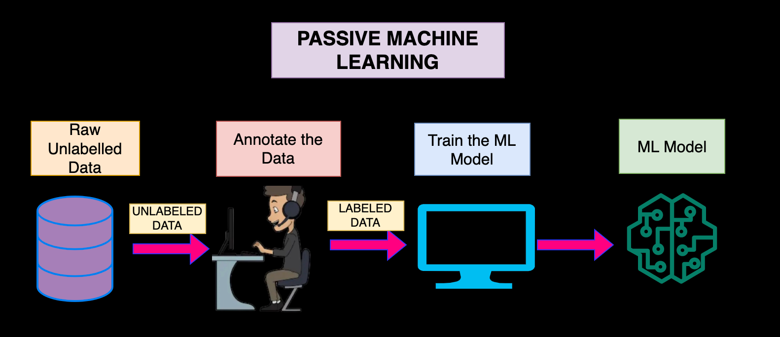
Imagine, instead if we are able to provide the machine learning algorithm with data points that capture most information then we can build a model with fewer data points (think of it as, if in a class you are taught the most difficult problems, you can use those concepts to solve the easy ones as the hard ones will most likely cover the important concepts).
With active learning, a machine learning algorithm can scan unlabeled training data and identify only the most useful data points for analysis. The program can then actively query either a labeled dataset or a human annotator (also known as the “oracle”) to label only those data points.

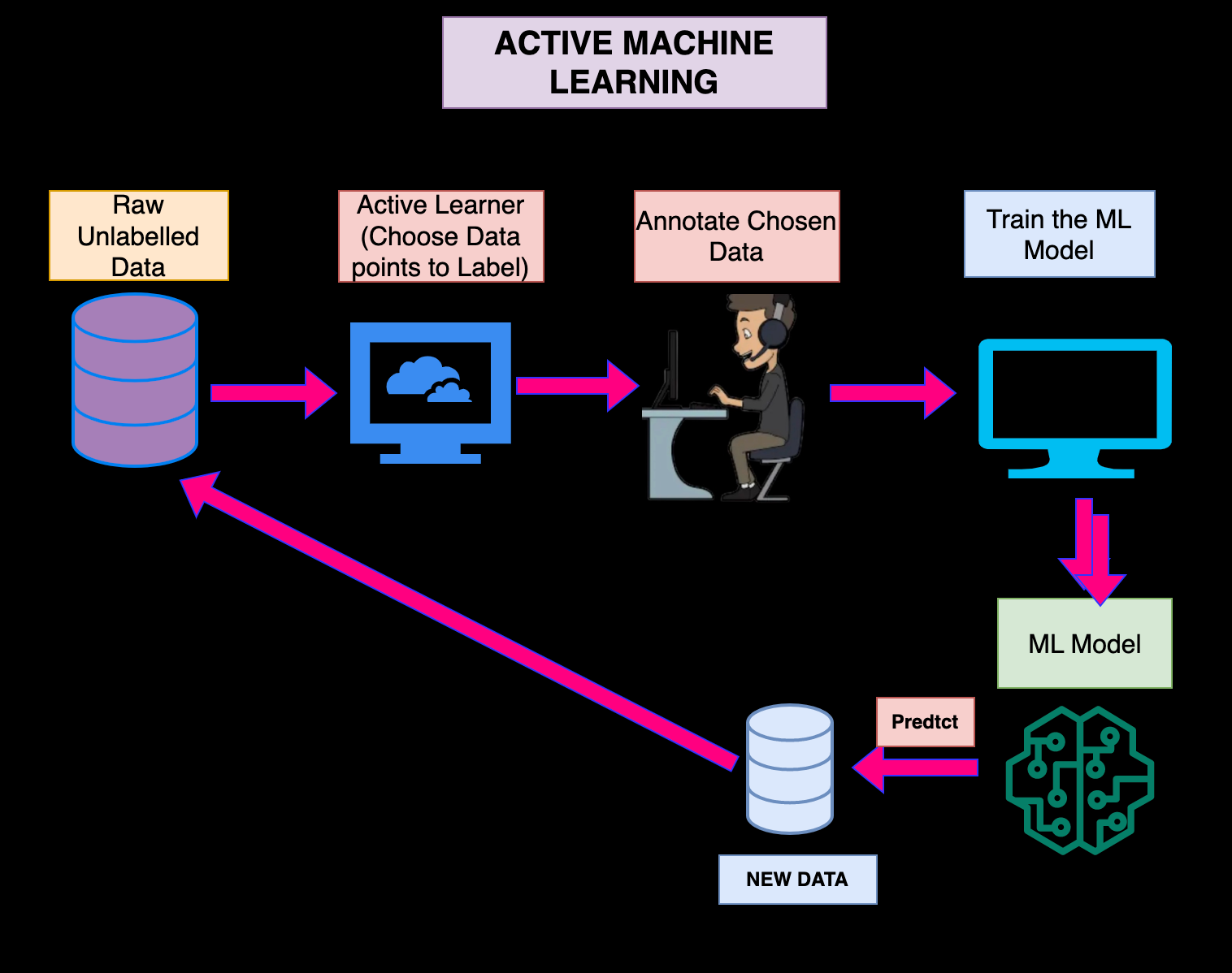
Active learning is a semi-supervised machine learning approach that allows models to be trained faster and with less data by discovering highly informative data points from unlabelled data.

Combining Active Learning with Deep-Learning Algorithms has shown tremendous potential by reducing training costs and also reducing the time to deploy AI applications. Active Learning also facilitates constant  retraining  based on incremental labelling updates.

Computer Vision models to detect product defects are a key application of AI in manufacturing. Traditionally, building such models needed large amounts of labeled data — In this article, I focus on how we can use Active Learning to build a Casting Defect Identification system with fewer labeled images and update the model by using newer data points that were not correctly classified by the model.

About the Data

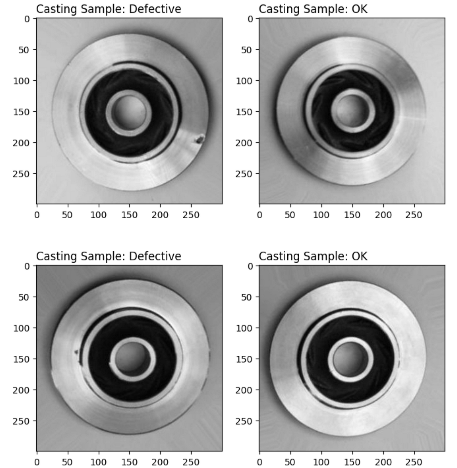
Casting is a manufacturing process in which a liquid material is usually poured into a mold and allowed to solidify. There can be defects like blow holes, pinholes, burr, shrinkage defects, mould material defects, etc. that occur during this process. A small defect in the casting process has a high impact on the quality of the final product. Traditionally, detecting these defects is a manual process that can be time-consuming.

In this article, we are going to use the data from Kaggle which contains top-view images of castings of a submersible pump impeller. The dataset contains 7348 grey-scaled images of size 300x300. The images are classified into two classes — ok and defective. The notebook to explore and visualize the data can be found here.

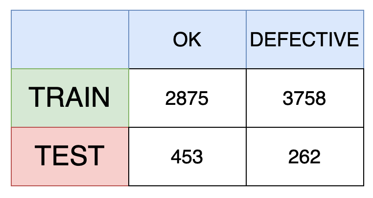
While this dataset has ~6K labeled data points in the train set — We will see that even with ~1000 images we can achieve around 90% accuracy in detecting defects.

The code, data, and the results of the experiments can be found in my Dagshub Repo

Our Approach

We going to iteratively build models on a smaller number of data points (starting from 100 images) and see how the model performs on test data. The test data is not used by the active learner but is used to measure the impact of Active Learning.

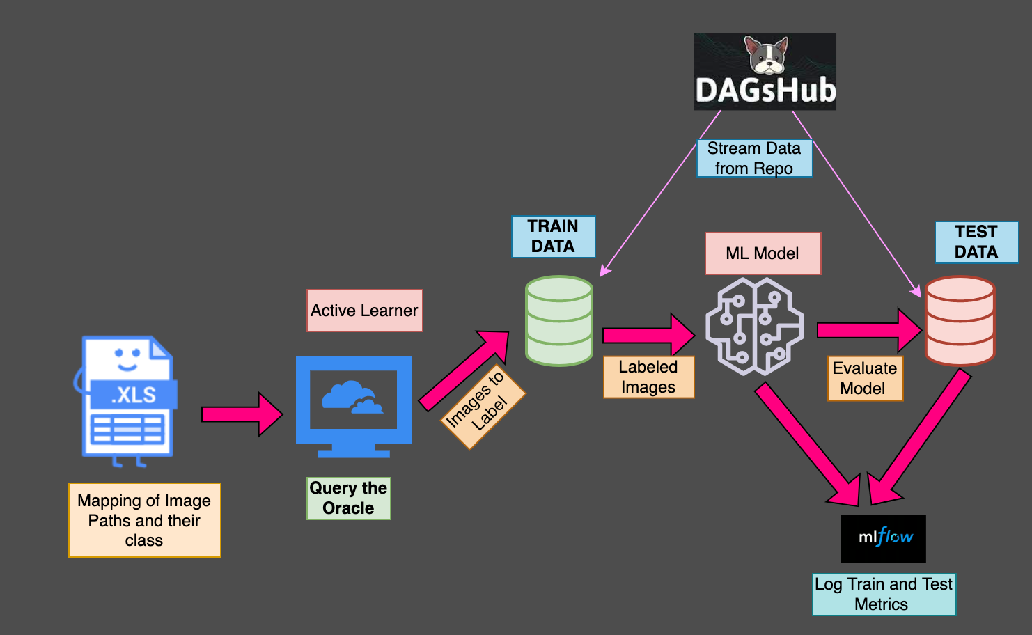
Since we do not need all the data at once, we are going to use the Dagshub Direct Access’s (DDA) streaming functionality to pull the data from the Dagshub Repo when needed. To understand more about Dagshub Streaming, refer to my article on Image Classification on Azure with Dagshub Direct Data Access. We are also logging the training parameters like the number of samples in the training data, the number of epochs, batch_size, etc,and the metrics on test & train data using MLFlow & Dagshub.

Integration of MLFlow and Dagshub allows us to track the code, data, and training parameters and metrics right from the Dagshub Repo.

Query the Oracle

Oracles in ancient Greece were priests who were mediums through whom advice/prophecy was sought. Similarly, in Active Learning, the human expert with domain knowledge who can help with the data labeling is referred to as Oracles. The Active Learner determines the data points that need to be annotated by the oracle

So, how does an active learner know which data points to choose for labeling? A simple way would be to randomly choose data points for labeling or we can use some measure of informativeness of a data point to choose the data to be labeled.

Random Query Strategy

As the name indicates, in this approach we will choose the data points randomly for labeling in every iteration. To know, how many datapoint to choose for labeling, we use the parameter “query_size”. In the first iteration, we generally use a random query strategy since we do not really know which data points are “informative” to the ML model.

def random_query_strategy(unlabelled_images,query_size):
    '''
    pick random samples from the unlabelled data for labelling
    
    '''
    images_to_label=random.sample(unlabelled_images,query_size)
    return images_to_label

Entropy-Based Query Strategy

Entropy is the measure of the uncertainty of a random variable. Entropy can be used as a proxy of the “informativeness” of data points. In this case, The most informative data points are the ones that the model is the least certain about. The idea behind is this that, the data points for which the model is less certain are the “hard” examples that contain the most information.

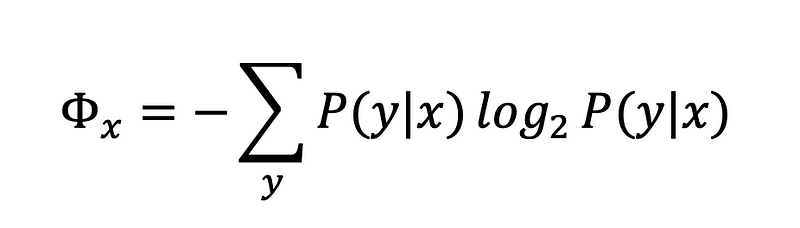
Here, P(y|x) is nothing but the probability of data point x belonging to class “y”. In our case, y can take two values 0 and 1.

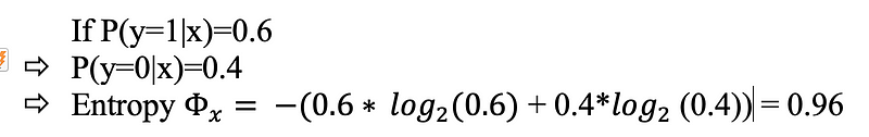
If the P(y=1|x)=0.5, then entropy is 1 indicating that the data point is close to the decision boundary.

Higher entropy means the data point is more informative or to put it in other words, model is not very sure which class the data point belongs to.

While using, the entropy-based strategy we pass the model as well because we are going to use the model to predict the probability score on the unlabelled images

The cleaned_images parameter in the function above is nothing but a dictionary containing the image path as the key and the NumPy array of the image (after pre-processing).

There are other querying strategies like Ratio Sampling or Least Confidence Sampling Strategy which like the Entropy Based Strategy use the prediction score as a measure of informativeness to choose data points to label.

def entropy_query_strategy(unlabelled_images,query_size,classifier,
                            cleaned_images=None):
    '''
    This function,gets the predicted probability of unlabelled images 
    and returns the images with the highest entropy for labelling

    cleaned_images is numpy array of the images that have been resized
    and converted to grayscale.
    '''
   
    image_pred_prob=predict_test_data(unlabelled_images,cleaned_images,
                                      classifier)
    
    image_pred_entropy={os.path.basename(file_path):entropy([prob,1-prob]) 
                      for file_path,prob in image_pred_prob.items()}
    
    ### Get the top N images with the highest entropy
    top_entropy=dict(sorted(image_pred_entropy.items(),key = 	itemgetter(1),reverse = True)[:query_size])
    print("Images to Label ",top_entropy.keys())
    return list(top_entropy.keys())

Building Active Learning Pipeline

This includes the following steps

1. Defining the Active Learner
2. Defining Image Data Generator to only choose images that have been picked by Active Learner for training
3. Test Image Data Generator that reads all the images in the test folder and processes them for prediction
4. Building the ML Model and Tracking the metrics on Dagshub+MLFlow.

The code for building this pipeline can be found in train_active_learning.py file

Defining the Active Learner

In this step, the active learner chooses from the set of images that have not been used for training (or unlabelled) using either a random or entropy-based query strategy. We are also keeping track of what images have been labeled. The Active Learner takes the classifier model as well as an input because, for entropy query strategy, we need to predict the probability of defect on the unlabelled data and choose the data points for labeling in the next iteration.

In the entropy-based strategy, before choosing the data points to label, we need to predict how the model performs on the unlabelled images in the training data and choose the data points based on the probability score. To speed up this process, instead of every time applying data pre-processing steps on the images, we create a dictionary of image paths and a NumPy array of the image after applying the pre-processing techniques in the first iteration and push this to the Dagshub Repo using the DDA upload functionality .

The code for this is defined in query_the_oracle() function in train_active_learning.py .

Let us pay a closer attention to the following lines from the query_the_oracle function shown in the code block below

if query_strategy=="entropy":
            
            if ITERATION_COUNT==1 and use_cleaned_array==False:
                ...
                ##1
                np.save('cleaned_images_numpy_array.npy',cleaned_images)
         
                ...
                ##2
                repo.upload(file="cleaned_images_numpy_array.npy",
                            path="cleaned_images_numpy_array.npy",
                            commit_message="Updating Cleaned Images",
                            versioning="dvc")

            if ITERATION_COUNT==1 and use_cleaned_array==True:
                
                ##3
                fs=create_streaming_client()
                numpy_file_path=os.path.join(DAGSHUB_REPO_NAME,     							           "cleaned_images_numpy_array.npy")
                fs.open(numpy_file_path)

                cleaned_images= np.load(numpy_file_path
                                        ,allow_pickle=True)
                cleaned_images=cleaned_images[()]
            
            CLEANED_IMAGES_ARRAY=cleaned_images
            ...

1. In the first iteration (ITERATION_COUNT=1 amd use_cleaned_array=False), we save the cleaned unlabeled images in the training data as numpy array and upload the numpy array to Dagshub Repo using DDA's upload functionality
2. When Iteration_COUNT=1 and use_cleaned_array=True, we use the DDA's streaming client to read the unlabeled training images which is stored as numpy array on the Dagshub Repo.

In both cases, once the numpy array is generated, we set the CLEANED_IMAGES_ARRAY global variable to enable persistence across iterations.This is done to save time in cleaning the data in the subsequent iterations.

Defining Image DataGenerator for Training (ActiveLearningDataGenerator class)

The data generator, reads and takes as input a  data file containing a list of paths of images in the training data that has been chosen for labeling by the Active Learner, the batch_size, the image dimensions, etc, and generates batches of data to be used for training the model. The data generator, instead of looking for files stored in your local machine, streams the necessary training images using the Dagshub Direct Data Access feature.

Defining DataGenerator for Test Data (DataGenerator class)

Even though ideally we use the same DataGenerator for test and train — I have defined them separately. The difference between them is that for the test data generator, we do not need to pass a data frame containing a list of image paths. Here, as well we read the test data from Dagshub Repo using the DDA's streaming feature.

Building and Evaluating the Model with Metrics Logging on Mlflow+Dagshub

To enable tracking the training parameters and metrics using mlflow, we set the tracking_uri as present in the Dagshub Repo and set the username and password as well.  

MLFLOW_TRACKING_URI="https://dagshub.com/AiswaryaSrinivas/"+DAGSHUB_REPO_NAME+".mlflow"
mlflow.set_tracking_uri(MLFLOW_TRACKING_URI)
os.environ['MLFLOW_TRACKING_URI']=MLFLOW_TRACKING_URI
os.environ["MLFLOW_TRACKING_USERNAME"] = MLFLOW_TRACKING_USERNAME
os.environ["MLFLOW_TRACKING_PASSWORD"] = MLFLOW_TRACKING_PASSWORD

To log, training metrics we use mlflow.tensorflow.autolog(). In addition, we also log the number of training data samples used to build the model.

As part of building the model, we also evaluate the model on the test data and log metrics like accuracy, precision, and recall in mlflow. This is defined in building_model() function in the train_active_learning.py

Putting it all together

To understand the impact of Active Learning we run the following steps till a stopping criterion is met. In our case, the stopping criterion for iterative training is till we have hit 3500 data points labeled by the active learner (this is a parameter called — threshold_sampling that is passed to the training code).

1. Call the Active Learner. If the entropy query strategy is used, this will predict the probability score on the unlabelled data in the training dataset and choose samples to label for the next iteration.
2. Train the model on the labeled data and Evaluate on Test Data

To run these steps from Google colab, refer to this notebook

The training can be run iteratively as below:

! python Casting_Defect_Identification/src/train_active_learning.py 
          --experiment_name="active-learning-entropy-v3"  
          --query_strategy="entropy" --n_epochs=10 
          --threshold_sampling=3500 --initial_query_size=100 --query_size=150

Here, query_strategy can take two values — random or entropy. The threshold_sampling acts as a stopping criterion (once 3500 images are labeled, the training stops), initial_query_size is the initial number of samples to label and query_size is the number of images to choose for labeling in the subsequent iteration.

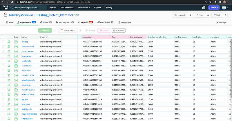
Results of Active Learning Experiment

The logged results can be seen both on MLFLow UI as well as on Dagshub Experiment Tab.

We used the following parameters — num_epochs=10, batch_size=16, and started with an initial sample size of 100 images and in every iteration, 150 new images were chosen for labeling by the Active Learner. All of these in captured in MLFlow and can be checked in the Experiments Tab in Dagshub.

Just to compare the two strategies, we plotted the Test Accuracy of the Random and the Entropy Based Strategy for different training sample sizes.

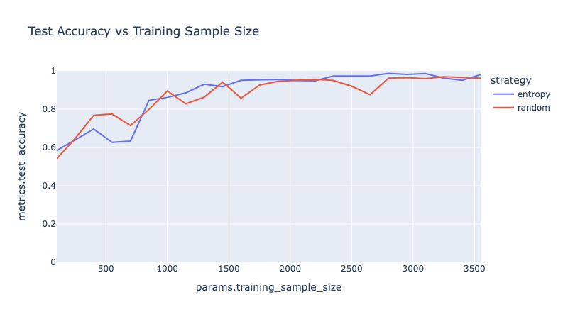
1. In general, the entropy-based strategy seems to perform better than the random strategy approach.
2. In the initial few iterations — the random strategy performs better than the entropy-based strategy, but once enough samples have been labeled using the informativeness of the data point can help in reducing the amount of data used for training, which in turn can reduce the training time as well.
3. We reach ~98% accuracy in detecting defects with 3500 samples in the entropy-based strategy and 95% accuracy in the random strategy.

In an entropy-based approach if there are a lot of similar images that are misclassified then all of them may have very high entropy and hence be picked for labeling in the same iteration — this can be avoided with a random strategy.

One can even use a combination of these strategies as well.

Registering the Model

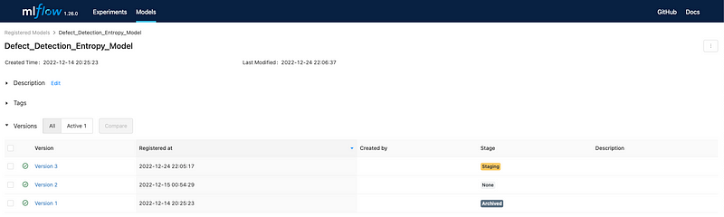
As a next step, we can register the model with the best results (the last iteration of Entropy Based Active Learning which resulted in 98% accuracy) on MLFlow. This can be achieved, directly using the UI or through code.

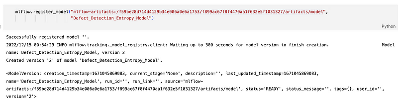
The model above has been registered in the name of “Defect_Detection_Entropy_Model”. Any newer models can be registered in the same name but the version number will change. This allows us to have model versioning as well.

Once the model is registered, we can use that model for predictions — by loading the model using the model_name and version

## Load the Defect Detection Model for predictions
import mlflow.pyfunc
MODEL_NAME="Defect_Detection_Entropy_Model"
MODEL_VERSION=3
model = mlflow.pyfunc.load_model(
    model_uri=f"models:/{MODEL_NAME}/{MODEL_VERSION}"
)

Conclusion

Machine learning models require a significant amount of data for their training process, which means a lot of time and resources are spent on labeling data. Active learning can help in reducing labeling costs and also one can have a baseline model up and running with a small sample of annotated data. Active Learning is a heavily under-utilized technique that can bring a lot of value to projects in industries like Manufacturing, where there can be a scarcity of labeled data. Here, we saw that with a simple CNN model and ~1000 images for training, we were able to reach 90% accuracy. With Active learning, as we see new images we can have a human manually label those images that the machine is not confident about and retrain the model.

In this article, we had labeled data already but if we wanted to build an interactive application that allows us to predict the probability of defects on newer data and annotate them, then we can use Dagshub LabelStudio.

In the next article, we will see how we can build an app and integrate it with Dagshub Label Studio to build a real-time active learning application.

Additional Resources

1. Project Repository on Dagshub
2. Active Learning — Theory
3. Experiment Tracking on Dagshub+MlFlow
4. Image Classification on Azure with Dagshub Direct Data Access