Build an End-2-End Active Learning Pipeline: Part 2
- Yono Mittlefehldt
- 9 min read
- 4 years ago

This 2-part tutorial will teach you how to implement an active learning pipeline using open source tools, such as MLflow, Label Studio, and DVC. You find part one here.
Welcome back!
In the previous part of this tutorial, we setup a REST API to serve our model and hooked it up to Label Studio. We then had Label Studio kick off predictions on our unlabeled data.
In this part, we’re going to finish the pipeline by:
- Annotating some of our data (but not all of it!)
- Streaming the annotated data to our training run
- Uploading our new model to the repo
All of this put together is a single cycle of our Active Learning Pipeline. Then it’s just a matter of repeating until we’re happy with our model.
Ready to continue?
Step 5: Annotating
Now that we have predictions for our data, we need to do something with it.
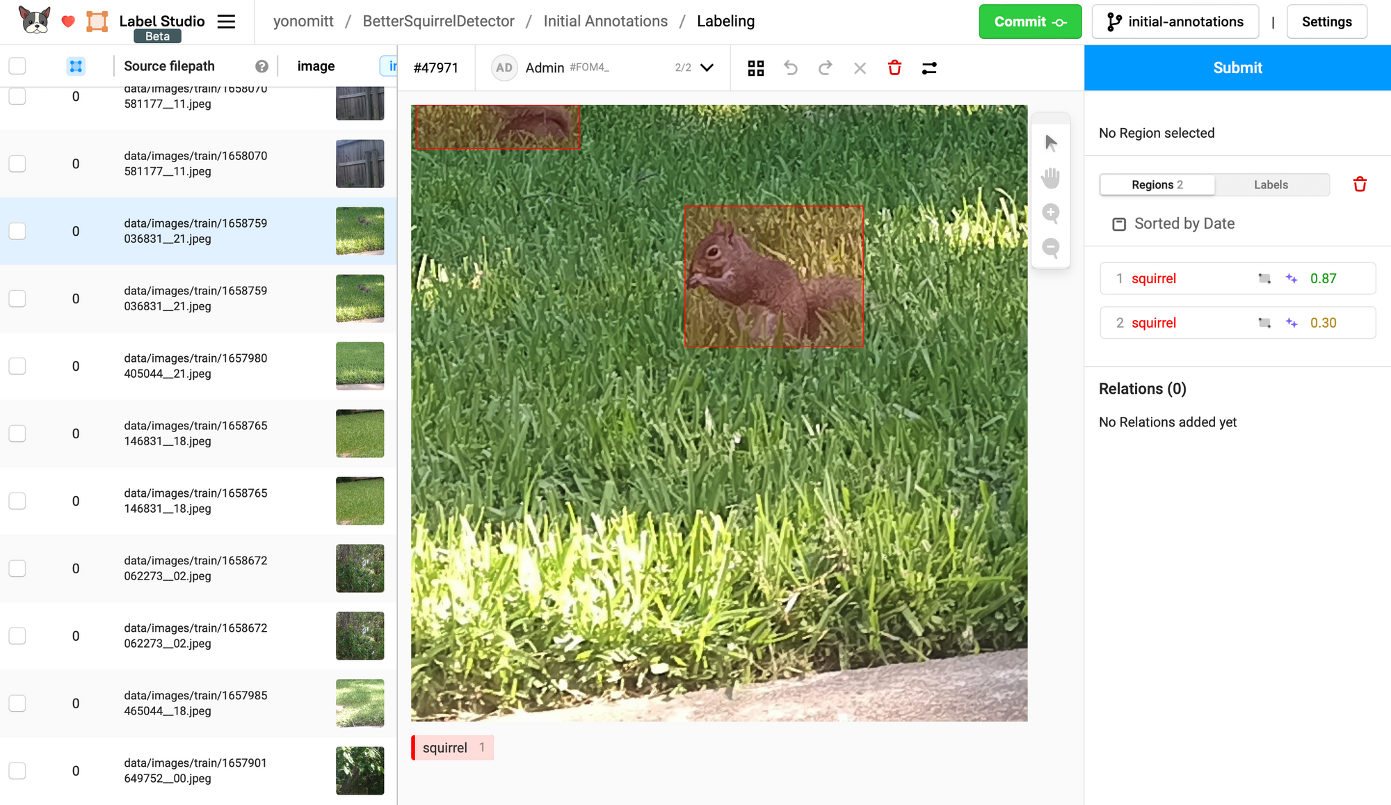
The first thing we want to do is sort our annotations tasks by Prediction score. To the right of the Order label, there is a button with a drop-down menu that allows us to select the column to sort by. Click it and select Prediction score.
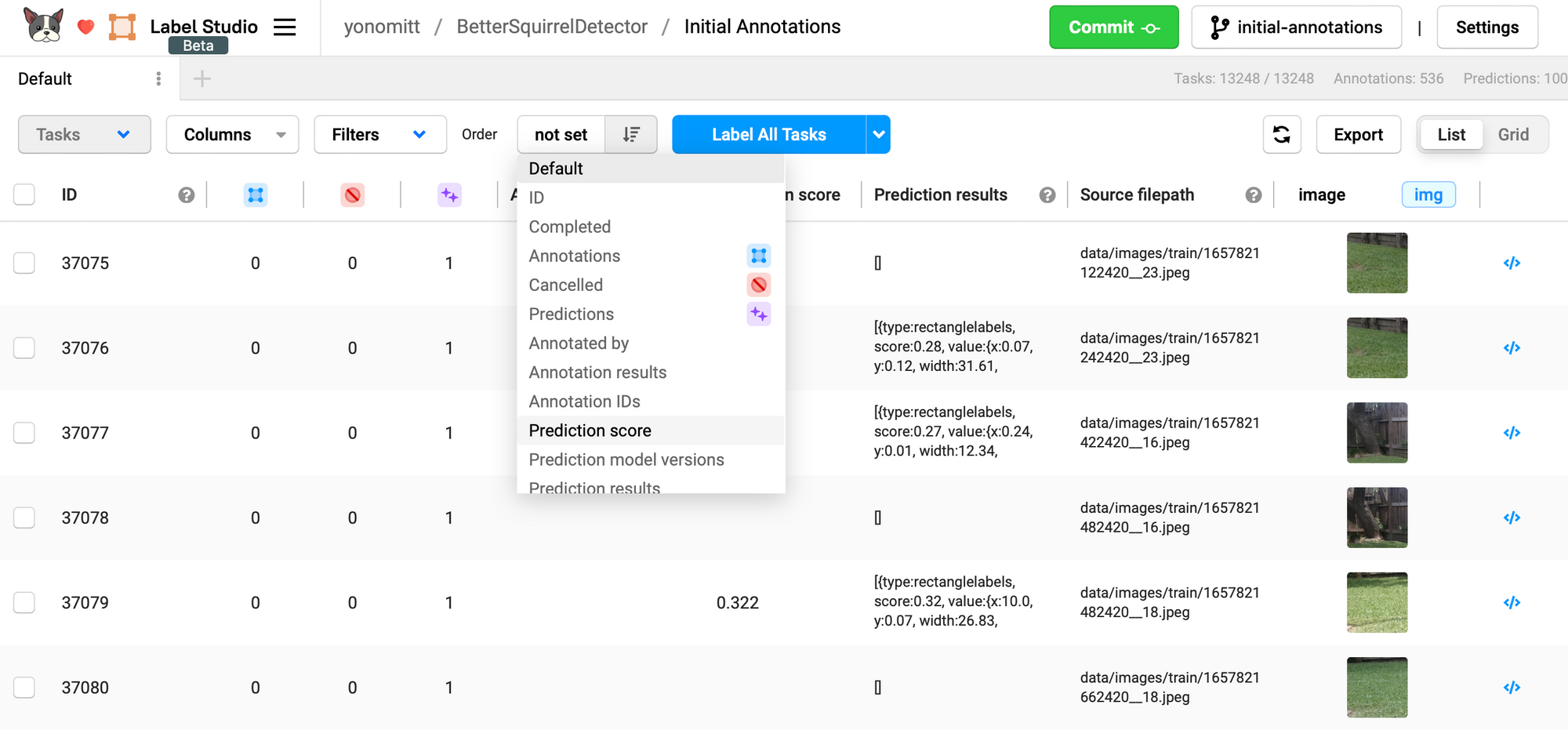
Since we want to focus on the images the model was least confident about, we’ll sort the tasks in ascending order of Prediction score.
If we wanted to use a different metric for the Prediction score, like estimated loss, we would want to sort it in descending order.
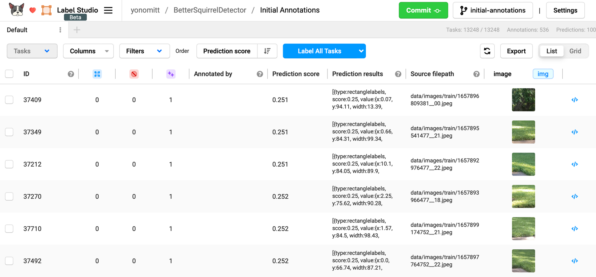
We’re now ready to start correcting the annotations predicted by our model. Starting at the top with the least confident predictions and working our way down to more and more confident predictions.
Sometimes these annotations will be false positives, which we need to delete. Other times there will be bounding box alignment that needs to be tweak. After each change, make sure you click the Submit button (but not the Commit button yet!)
Since we’re creating an active learning pipeline, we don’t want to go through and fix all annotations. That would defeat the purpose. So how many do we want to fix in each cycle?
That is a tough question and will also be very project dependent. If you pick too few, you’ll end up iterating on your model too often. However, if you pick too many, you run the risk of annotating more than you needed to and wasting time, money, and effort.
We can either choose a threshold prediction score, a fixed number of images, or a combination. For instance, we could choose a threshold but do, at most, a certain number. This is the human element of active learning.
In the case of the squirrel detector, we’re using YOLOv5. The current model we’re using was trained on about 240 images. So for our initial cycle of active learning, I suggest we try annotating a maximum of 50 images and see how much that improves our model.
In later active learning cycles as our model becomes more accurate, we may need our training to focus on even harder examples to squeeze out more improvements. This may require more sophisticated algorithms to ensure the toughest samples are chosen without selecting outlier data.
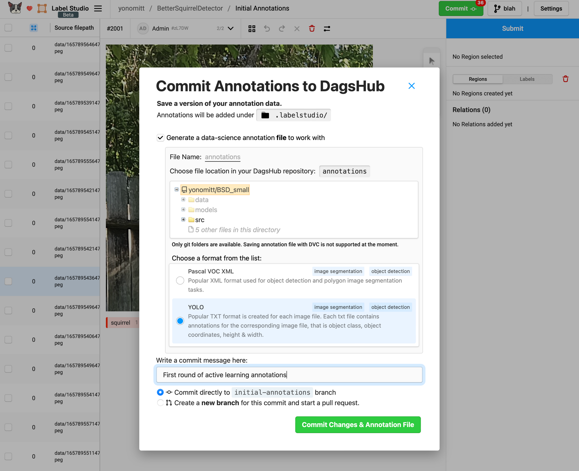
When you’re done annotating, you can Commit the annotations to the repo. When you do this, Label Studio gives you the option to also generate annotation files in different formats. Since we’re using a YOLOv5-based model, it makes sense to select the YOLO format. Label Studio will only generate annotation files for the images you updated, not for all images with predictions, which is exactly what we want.
For this project leave the File Name and file location for the YOLO annotation files as the defaults.
Go ahead and annotate some images and then come back for the next step.
Step 6: Train a New Model
Now that we have some annotations, it’s time to train a new model.
However, since we’re only training on a small fraction of the data, ideally we don’t want to have to dvc pull down the entire dataset to our machines. That would be a waste of time. This is where the new Data Streaming Client can help us!
The Data Streaming Client allows us to pull down data as we need it. Additionally, it saves the streamed data locally, so we’re not required to download the same images for each epoch.
Using the Data Streaming Client is easy! First you need to install the DagsHub Python library:
pip install dagshubThen, at the top your Python script, add the following:
from dagshub.streaming import install_hooks
install_hooks()
This function monkey patches various file system related methods (os.open, os.scandir, etc), which means data will automatically be streamed or read locally depending on the situation. For more information, check out this introductory post.
If you take a look at the main function in the train_squirrel_detector.py script, you’ll see that we need to do some setup in order to run YOLOv5 from our repo:
# 1
temp_yolov5_path = 'yolov5'
download_training_scripts(temp_yolov5_path)

# 2
_ = torch.hub.load('ultralytics/yolov5', 'custom', path=args.weights)

# 3
import utils

# 4
utils.dataloaders.img2label_paths = custom_img2label_paths
With this code, we:
- Download the YOLOv5 train.py and val.py scripts to a temporary directory.
- Take advantage of a side effect of calling
torch.hub.loadto download and cache the YOLOv5 repo. This will make it’s submodules and functions available to our scripts. - Import YOLOv5’s
utilssubmodule. - Monkey-patch YOLOv5’s
img2label_pathsfunction with our own custom implementation. This is necessary because YOLOv5 expects images and labels in the datasets to have very specific and parallel structures. However, Label Studio doesn’t follow this when exporting YOLO annotations. Our custom function converts our dataset image paths to Label Studio’s exported annotation paths.
Next we have some code that monkey patches around a feature (or a bug depending on your point of view) of YOLOv5. The problem is that if an image doesn't have a corresponding annotation file, YOLOv5 will still use the image for training but assume there are no objects in the image. This means it will still download our entire dataset and train with a bunch of really bad data.
To fix this, we create a new function that monkey patches the utils.dataloaders.LoadImagesAndLabels.cache_labels used by the data loader. This function deals with caching labels for quicker access. However, our version will remove ensure that only images we've labeled are included in the dataset.
# 1
orig_cache_labels = utils.dataloaders.LoadImagesAndLabels.cache_labels

# 2
labeled_imgs = get_labeled_images()

# 3
def custom_cache_labels(self, path=Path('./labels.cache'), prefix=''):
    data_cnt = len(self.im_files)
    for i in reversed(range(data_cnt)):
        im_file = self.im_files[i]
        _, im_name = os.path.split(im_file)
        if im_name not in labeled_imgs:
            self.im_files = self.im_files[:i] + self.im_files[i+1:]
            self.label_files = self.label_files[:i] + self.label_files[i+1:]

    # 4
    return orig_cache_labels(self, path, prefix)

# 5
utils.dataloaders.LoadImagesAndLabels.cache_labels = custom_cache_labels
Here we:
- Store a copy of the original
cache_labelsmethod. - Call our function to extract the file names for all images that were annotated in Label Studio (in the same train_squirrel_detector.py script)
- Create a custom version of the label caching method, which first removes any images and corresponding annotations that are missing from our
labeled_imgsset... - Remember to call the original
cache_labelsmethod we stored, so we get the correct functionality when training. - Monkey-patch YOLOv5's
cache_labelsmethod with our custom version.
With both of those methods successfully patched, we can finally get to the actual training code:
# 1
train = importlib.import_module(f'{temp_yolov5_path}.train')

# 2
train.run(weights=args.weights,
          data=new_yaml,
          hyp='data/hyps/hyp.scratch-low.yaml',
          epochs=args.epochs,
          batch_size=args.batch_size,
          name='squirrel',
          exist_ok=True)
This training code:
- Imports the YOLOv5 training script we downloaded, which loads our monkey-patched functions, and...
- Starts a training run using our script's parameter.
When training is done, there is some code to move our model to the specified path and clean up the training run files.
We can run this script using the following command:
python train_squirrel_detector.py --data data/squirrels.yaml \
                                  --weights ../models/model3_finetune.pt \
                                  --save-path ../models/model4_loop0.pt
This command will use our pre-trained model as a starting point and save the resulting trained model in our repo’s modelsdirectory.
We’ve almost finished our first active learning cycle. There is just one more thing left to do before we start the cycle over again… and it’s super easy.
Step 7: Upload the Model to the Repository
We want to add our newly trained model to the our repo. The old way would be to use dvc add
followed by dvc push. However, DagsHub has a new trick up its sleeve. There is now an Upload API to complement the Data Streaming Client. And it’s simple to use.
When you installed the dagshub Python library, it also installed a Command-Line Interface (CLI). Let's use this CLI to upload our new created model.
The general command looks like this:
dagshub upload [--branch BRANCH] <repo_owner>/<repo_name> \
               <local_file_path> <path_in_remote>
For our case we'll run:
dagshub upload --branch initial-annotations \
               yonomitt/BetterSquirrelDetector \
               model4_loop0.pt \
               models/model4_loop0.pt
After following the instructions to authenticate yourself, this will upload the model4_loop0.pt file to the models folder in the repo.
Nice!
Step 8: Rinse and Repeat
At this point, we’ve now completed an entire cycle in our active learning pipeline. It’s now time to repeat this cycle until we’re satisfied with our results.
Go back to Step 1 and this time, register the model you just finished training to the MLflow Model Registry using the register_model.py script.
If you use the same model name when registering, MLflow will automatically increment the version number for the model. This means, the scripts from Step 2, which runs the model in the web server will work without any edits. However, you still need to rerun the docker-compose command or you’ll be using your old model!
You should be able to skip Step 3 in subsequent cycles, as Label Studio should already be set up for you, unless you want to create a separate Label Studio project per cycle.
Whoever said you shouldn’t repeat yourself?!?
Results
To put some concrete data behind this active learning pipeline for this project, here are the results we got after running through several cycles:
| Model | Precision | Recall | mAP@0.5 | mAP@0.5:0.95 |
|---|---|---|---|---|
| model3 | 0.919 | 0.615 | 0.741 | 0.513 |
| model4 (loop 0) | 0.95 | 0.901 | 0.937 | 0.734 |
For these results, we manually created and annotated a test set that was kept constant throughout all cycles to give a fair apples-to-apples comparison.
So how do we know how many iterations are enough? Unfortunately, much like the question about how many images should be annotated, this is going to depend on the project. You’ll likely notice that on average, the lowest confidence scores start to increase the more cycles you run. This will often coincide with less and less improvement on model accuracy, too.
Conclusion
Wow! You’ve made it to the end of these tutorials. Fantastic! You’ve learned a ton about creating an active learning pipeline using some pretty powerful tools.
- MLflow - registered models to and loaded models from the Model Registry
- Label Studio - used to run predictions and annotate data
- DVC - the streaming client and upload API use DVC under the hood!
- DagsHub - platform that integrated all of these tools
- Streaming Client - pulled just the data needed for the current training run
- Upload API - committed newly trained models to the repository
By using active learning in your projects, you can decrease the time and cost of labeling data. Additionally, it’s possible to improve your models’ accuracies by having them learn from the hardest training samples.
CHALLENGE - Using this post and sample project repo as a starting point, create your own active learning project and share it with us on Discord and Twitter! We’d love to see what you can do!
If you have any questions, feel free to reach out.