Build an End-2-End Active Learning Pipeline: Part 1

This 2-part tutorial will teach you how to implement an active learning pipeline using open source tools, such as MLflow, Label Studio, and DVC.

Psst 🤫

You. Yeah, you!

Want to hear a secret?

Focusing on the data is at the heart of data-centric AI. And although it might not be as glamorous as inventing a new algorithm or model architecture, if often is the best bang for your buck.

One very important technique within data-centric AI is Active Learning. Active learning not only allows you to improve your model’s accuracy, but to do it with less data. This means you save time and money on the labeling side as well as on the training side! It also allows you to get to production faster, since you spend less time on the initial model. 😎

However, setting up an Active Learning Pipeline is rather challenging. It generally requires you to either do a lot of manual work, which is prone to error, OR requires you to be an expert in many areas of MLOps. Many people want to implement active learning, but only leading teams tend to succeed. But what if it didn’t have to be hard anymore?

This 2-part tutorial will show you how to set up an end-to-end Active Learning Pipeline based on open source tools.

In part one, you’ll learn how to:

1. Serve a machine learning model via a REST API
2. Connect your machine learning backend to Label Studio
3. Run predictions on your unlabeled training set

Next, in part two, you’ll complete the pipeline and learn how to:

1. Decide which data should be labeled
2. Stream just the labeled data to your training runs
3. Train a new model, which can be used to start the active learning loop again

After going through both tutorials, you will be able to implement a similar pipeline for your machine learning projects and use it to improve your models!

What are we waiting for? Let’s get started!

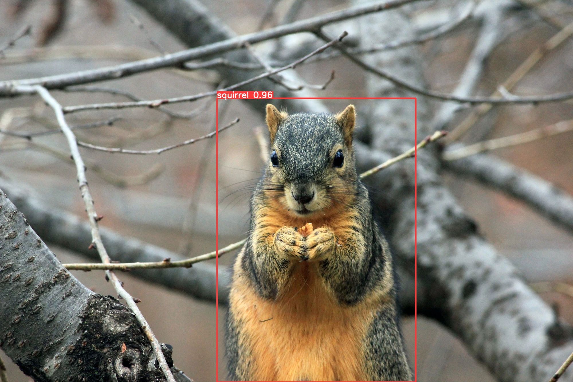
Return of the Squirrel Detector

In a previous post, we created a Squirrel Detector and iteratively improved its accuracy metrics just by cleaning up our data. While you don’t need to read that article, it might provide better context as you go through this one.

In that project, we collected the data by scraping images from DuckDuckGo, which tends to favor high-quality, close-up images of squirrels. Due to this, our Squirrel Detector is very good at detecting squirrels in very clear images.

However, if we setup the model on a Raspberry Pi connected to a webcam and point it at our backyards… we may be disappointed in the results. This is because these images are too different from the scraped images. They fall outside the distribution of our training data.

How do we solve this? We need to fine-tune it on data captured by webcams!

Over the course of a month, I setup a webcam and captured over 12,000 4k images of a backyard with and without squirrels. In order to better work with our YOLOv5 model, we can tile each of those images into 24 pieces. This results in about 300,000 images to train, validate and test with!

Tiling has the added benefit that any squirrels captured in the images would be a larger percentage of the image, making them easier to detect.

However, now we have another problem. We have way too much data to annotate by hand in a reasonable time OR for a reasonable cost.

Luckily, Active Learning can help us solve this problem!

Let’s take a look at the active learning pipeline we’re going to implement.

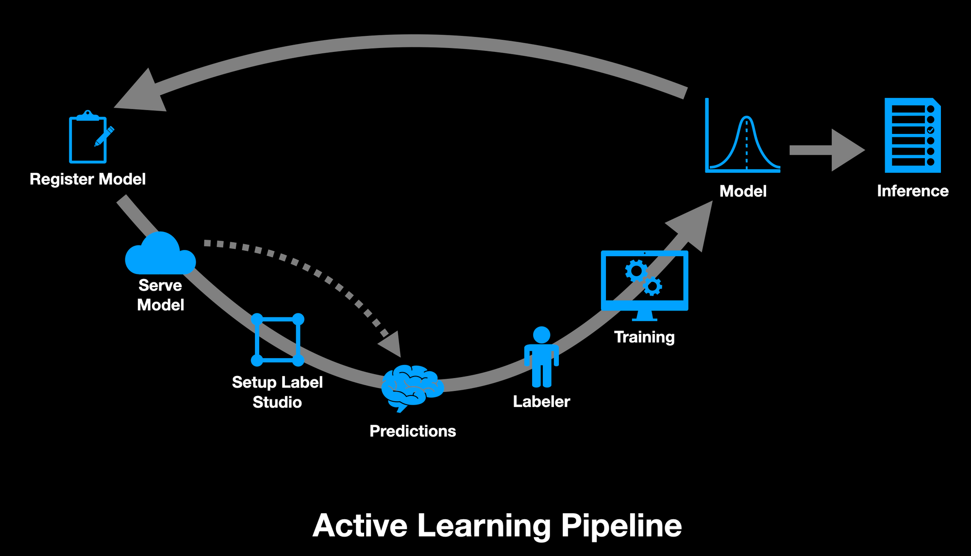
From this diagram, you can see that we need to:

1. Register a model to the MLflow Model Registry
2. Serve the model behind a REST API compatible with Label Studio
3. Setup a Label Studio annotation project and configure it to use our model
4. Have Label Studio run predictions on all data
5. Sort the data by prediction score and manually correct and commit the annotations for the top images
6. Train a new model
7. Upload the model artifact to the repository
8. Rinse and repeat!

Excited yet? Then let’s get started!

Step 1: MLflow Model Registry

We need to start our active learning pipeline by registering a model to our repo’s MLflow Model Registry. This will make it much easier to keep track of all our models AND allow us to load and serve them later in our pipeline.

In the BetterSquirrelDetector repo, we have a few helper scripts to register an existing YOLOv5 model to the repo’s MLflow Model Registry.

There are a few steps we need to follow. First, we need a way to create or get an MLflow experiment by name. This is exactly what the get_experiment_id function in get_or_create_mlflow_experiment.py does:

import mlflow

def get_experiment_id(name):
    exp = mlflow.get_experiment_by_name(name)
    if exp is None:
      exp_id = mlflow.create_experiment(name)
      return exp_id
    return exp.experiment_id

Next, we need a wrapper class for our model that inherits from mlflow.pyfunc.PythonModel. This wrapper class can be found in model_wrapper.py:

import mlflow
import torch


class SquirrelDetectorWrapper(mlflow.pyfunc.PythonModel):
    def load_context(self, context):
        self.model = torch.hub.load('ultralytics/yolov5', 'custom', 
                                    path=context.artifacts['path'])

    def predict(self, context, img):
        objs = self.model(img).xywh[0]

        return objs.numpy()

In order to conform to mlflow.pyfunc.PythonModel, the wrapper class needs to implement the predict function for inference. It can also optionally implement the load_context model to do any setup work.

During setup, this model wrapper loads a custom YOLOv5 model from a path passed in via the context.

After running inference, it converts the output of the model to a numpy array of bounding boxes.

The register_model.py script uses both of these pieces to register our model to the Model Registry using the MLflow API:

...

exp_id = get_experiment_id(args.name)

with mlflow.start_run(experiment_id=exp_id):
    mlflow.pyfunc.log_model(
        'finetuned',
        python_model=model,
        conda_env=conda_env,
        artifacts=artifacts,
        registered_model_name=args.model_name
    )

With all that in place, what model are we going to register? We haven’t even done any training, yet!

If you recall, we have a decent squirrel detector model already. Why not start with that one? The BetterSquirrelDetector repo includes the final trained model from the SquirrelDetector repo.

To register this model, we can run the script like so:

python register_model.py --name SoManySquirrels \
                         --model ../models/model3_finetune.pt \
                         --model-name SquirrelDetector

Where:

• name is the experiment name to use
• model is the path to the model artifact to register
• model-name is the name to register the model under

We need to remember what we choose for the model-name. This will be important when we’re ready to serve our model.

If you’re interested in more in-depth information on MLflow, checkout out our two-part MLflow Crash Course where we cover all this and more in detail:

• What is MLflow and MLflow Tracking
• Model Registry and Model Deployment

Step 2: Serve the Model behind a REST API

If you’re familiar with MLflow, you might be thinking you know where this is going. We just need to serve or deploy our model using MLflow’s built-in features!

Unfortunately, it’s not that simple this time.

The problem here is a misalignment between how MLflow deploys models and how Label Studio expects to reach models. MLflow uses a hardcoded endpoint /invocations to run inference on the models. However, Label Studio expects to send data to an endpoint called /predict.

So instead of using MLflow to serve our model, we’ll have to create our own web server compatible with Label Studio. However, we can still use MLflow to load the appropriate model from within our web server!

Check out the src folder in the BetterSquirrelDetector repo. Here we find several files related to running the web server:

• ls_model_server.py - Contains the SquirrelDetectorLSModel class. It includes a predict method, which is run when the /predict endpoint is called.
• Dockerfile - This is the Dockerfile that builds the web server image.
• docker-compose.yml - Used to start up the web server and connect it to a local redis store. It includes passing environment variables from your current shell to the web server, in order to properly configure MLflow.
• _wsgi.py - A Web Server Gateway Interface that initializes the SquirrelDetectorLSModel and connects it to the web server.
• webserver/ - This folder contains configuration files needed to instantiate the web server and the ML model.

The most interesting code concerning our Squirrel Detector, is the SquirrelDetectorLSModel class found in ls_model_server.py. Specifically the __init__ and predict methods.

At the end of the __init__ method, we see:

# 1
mlflow.set_tracking_uri(os.getenv("MLFLOW_TRACKING_URI"))

# 2
client = mlflow.MlflowClient()
name = 'SquirrelDetector'
version = client.get_latest_versions(name=name)[0].version

# 3
model_uri = f'models:/{name}/{version}'

# 4
self.model = mlflow.pyfunc.load_model(model_uri)

With this code we:

1. Set our remote tracking URI for MLflow to point to our DagsHub MLflow server, which comes with every repo. This URI is being pulled from the environment variables passed into the docker-compose.yml file.
2. Get the latest version number of our model, named SquirrelDetector, from the MLflow Model Registry. Note that the name must match the one we registered the model under in Step 1: MLflow Model Registry.
3. Construct the model URL based on the model name and version number.
4. Load the model from the MLflow Model Registry.

The predict method, takes tasks from Label Studio as a parameter. It then calls the predict_task method for each one.

These tasks are lists of dictionaries, which include info about the data. Label Studio, however doesn’t send the raw images, but rather a URI describing them. So we need to first do a little work to get the actual images:

def predict_task(self, task):
    
    #1
    uri = task['data']['image']
    
    #2
    url = self.image_uri_to_https(uri)
    
    #3
    image_path = self.get_local_path(url)

Here we:

1. Extract the URI from the task, which is in the form of repo://<commit hash>/<path to image>
2. Convert the repo:// URI into a URL, from which we can download the image
3. Use a helper function to download the image to a local cache and return the path to it

After this, we can load the image and run inference on it!

The format that Label Studio requires for object detection models looks like:

[
    # One dictionary for each task/image
    {
        # list of dictionaries describing the detected objects
        'result': [
            {
                'from_name': self.from_name,
                'to_name': self.to_name,
                'type': 'rectanglelabels',
                'value': {
                    'rectanglelabels': [label],
                    'x': x,
                    'y': y,
                    'width': w,
                    'height': h,
                },
                'score': confidence_score
            },
            ...
        ],
        
        # a single, combined score for the predictions made for the image
        # this is extremely important for active learning
        'score': prediction_score
    },
    ...
]

The prediction_score we’ll use for our active learning use case is the lowest confidence percentage of any detected squirrels. This will later allow us to sort images by confidence level to help us decide which images we want to annotate.

At the end of predict_task, we have the following code:

# 1
url = f'https://dagshub.com/{self.user}/{self.repo}/annotations/git/api/predictions/'

#2
auth = HTTPBasicAuth(self.user, self.token)

#3
res = requests.post(url, auth=auth, json=result)

This code:

1. Constructs the Label Studio API URL to create a prediction for a task
2. Creates an HTTPBasicAuth structure to be used with our API call
3. Calls the API URL using the POST method, passing in out authentication and prediction results

With all this code in place, we can start our web server by running:

docker-compose up --build

The --build flag ensures we rebuild the application each time. This is really only necessary if you change the code within ls_model_server.py, if, for instance, you change the name of your MLflow registered model between active learning cycles. However, using it each time can potentially prevent hard to track down bugs, in which the wrong model is being used!

When finished, we have a web server running on port 9090!

Naturally, since we’re building docker images, we could easily deploy these to AWS or GCP, but we also have the option to run them locally, if we choose.

Step 3: Setup Label Studio

Next, we need to setup Label Studio to use our model to make predictions. Once we have the predictions, we can then make a choice as to which images we need to annotate.

From your repo on DagsHub, click on the Annotations tab and then click the Turn on Workspace! button. After doing so, we can see a spinner and a message telling us it should take a few minutes.

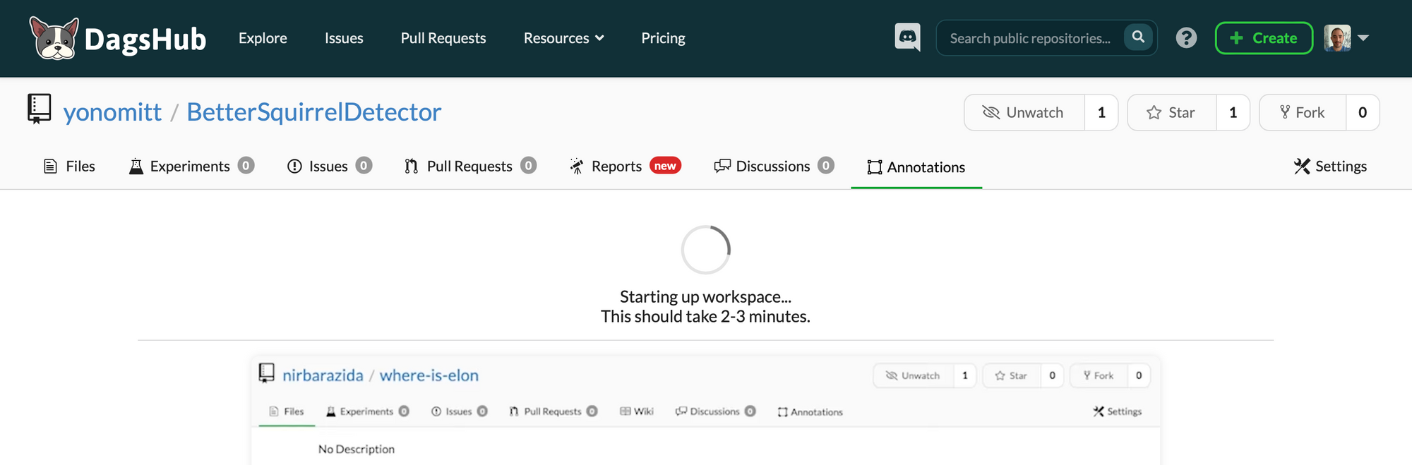
Time for a coffee break!

When that comes back, click the Ready button to bring up the Annotation projects page.

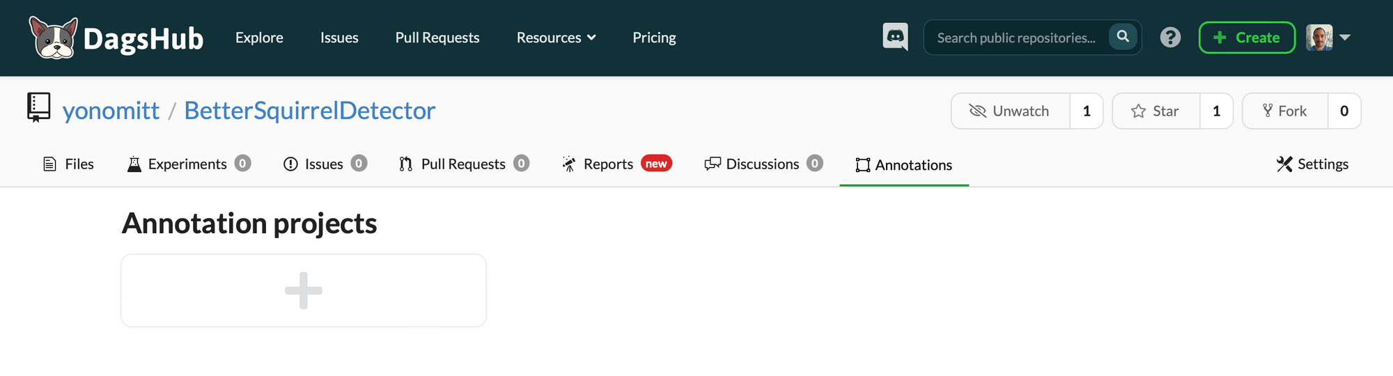
Click on the big plus button to bring up the New annotation project form.

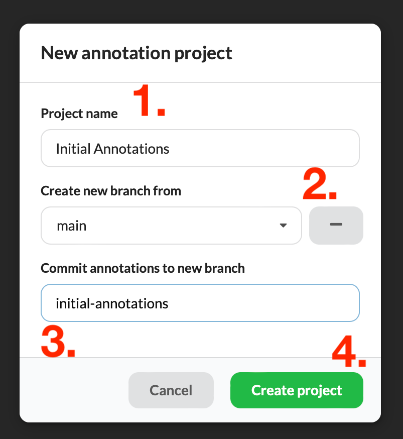
Here we want to:

1. Enter a project name
2. Click the plus button to create a new branch for our annotations
3. Enter a descriptive branche name
4. Click the Create project button

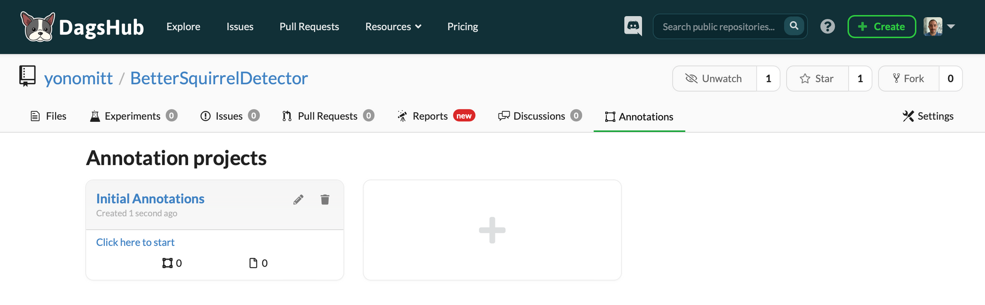
After clicking on the annotation project you just created, you should be presented with the project settings.

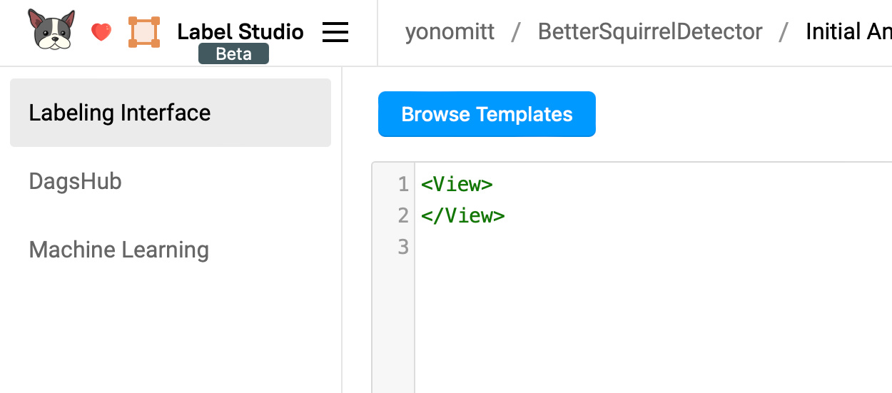
You need to enter these settings in a very specific order:

1. Labeling Interface
2. Machine Learning
3. DagsHub

If you don’t setup the Labeling Interface first, then the Machine Learning model setup will fail. The DagsHub settings can technically be done at any time, but it’s easiest to save it for last.

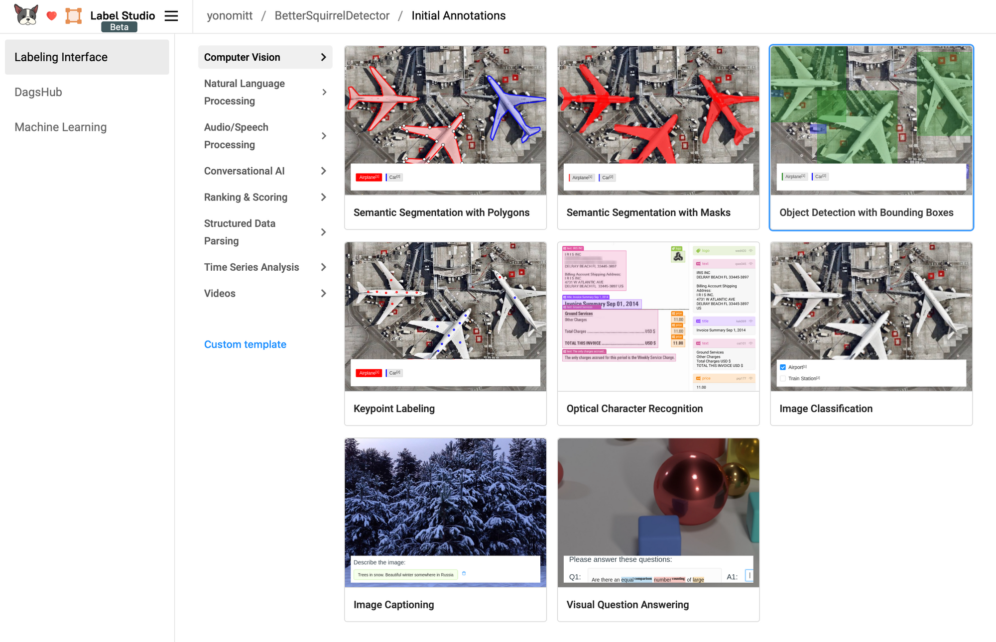
Let’s start by clicking the Browse Templates button under Labeling Interface.

With the Computer Vision category selected, click the Object Detection with Bounding Boxes template.

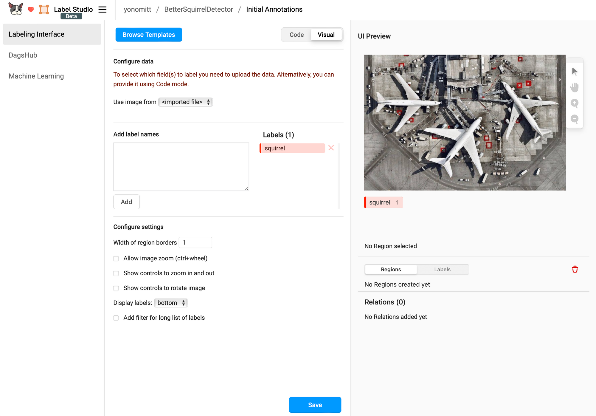
Remove the existing example labels for Airplane and Car and add a new one for squirrel. Feel free to choose a color of your liking, but just know that the images have a lot of brown and green in them. When you’re done, click Save.

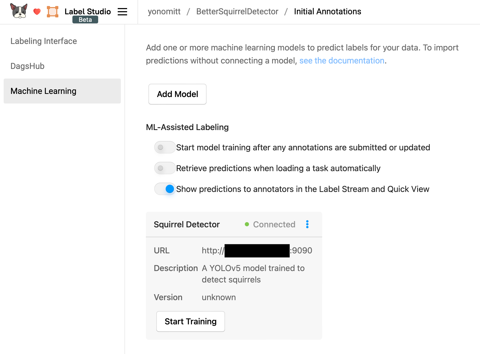
Next, we need to configure Machine Learning. Clicking on that will present you with the settings for your model.

Ensure that both Start model training after any annotations are submitted or updated and Retrieve predictions when loading a test automatically are turned off. If you leave these on, Label Studio will automatically send training and prediction requests to our server too often and when we don’t want it to. We want to remain in control!

Click the Add Model button to bring up the add model form.

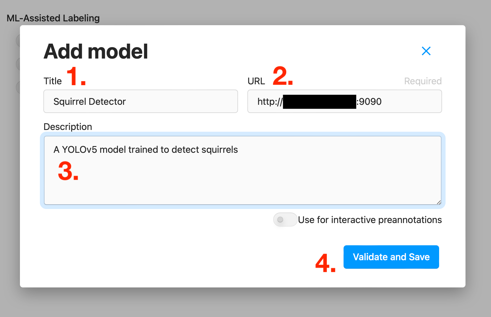
Here we want to:

1. Give our model a meaningful title
2. Enter the URL to our server including the port
3. Add a description for our model
4. Click the Validate and Save button

Label Studio will then make sure it can access the server, check that all expected endpoints are present, and save the model configuration.

Finally, we need to configure the DagsHub settings. Here we need to select the folder with all of our training data (for simplicity, the validation and test sets have already been annotated) and then click Save.

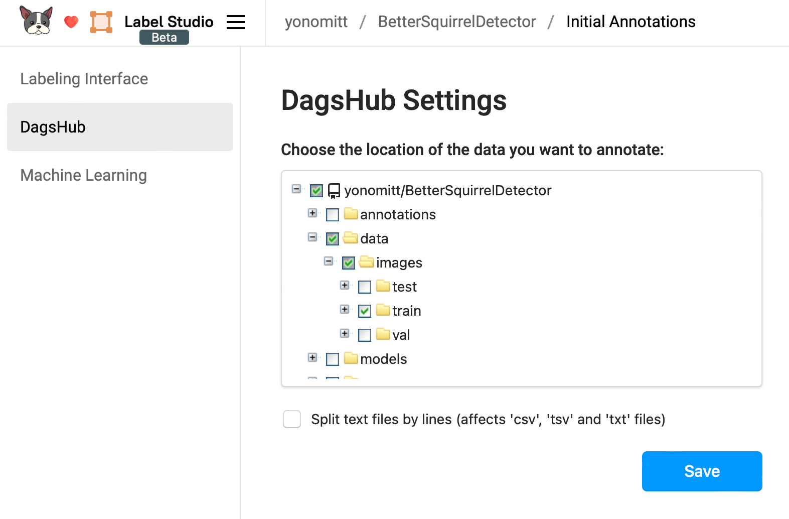
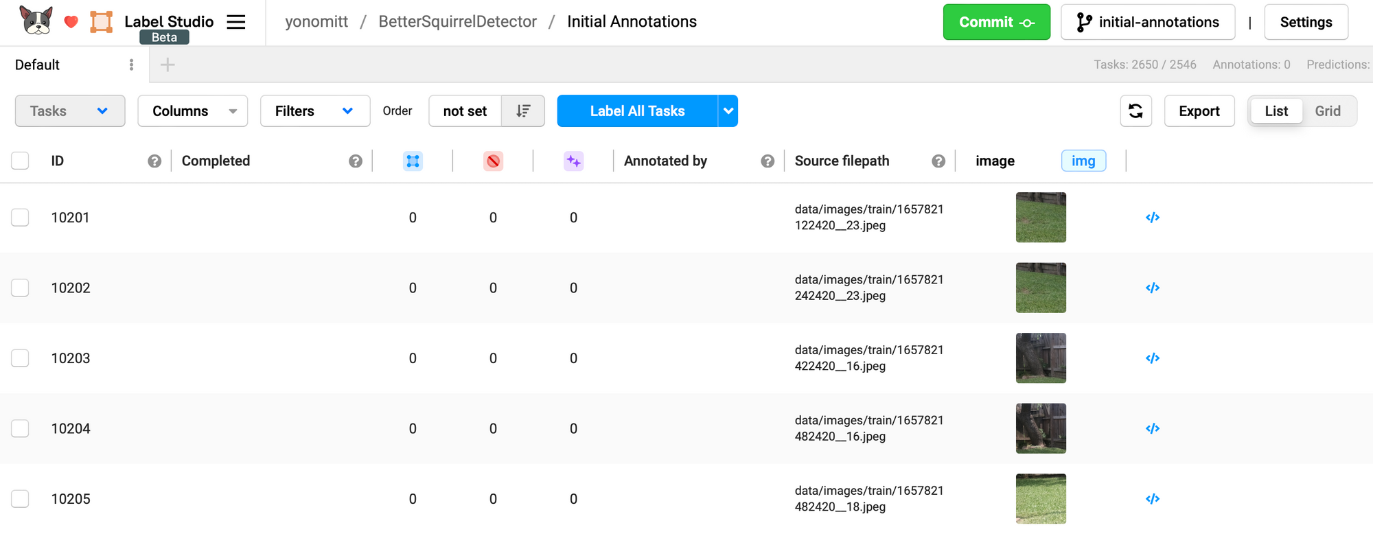
Once we’ve done that, we should be taken to the main Label Studio interface, which includes a list of all the data we’ve selected.

This leads us straight into the next step.

Step 4: Running Predictions

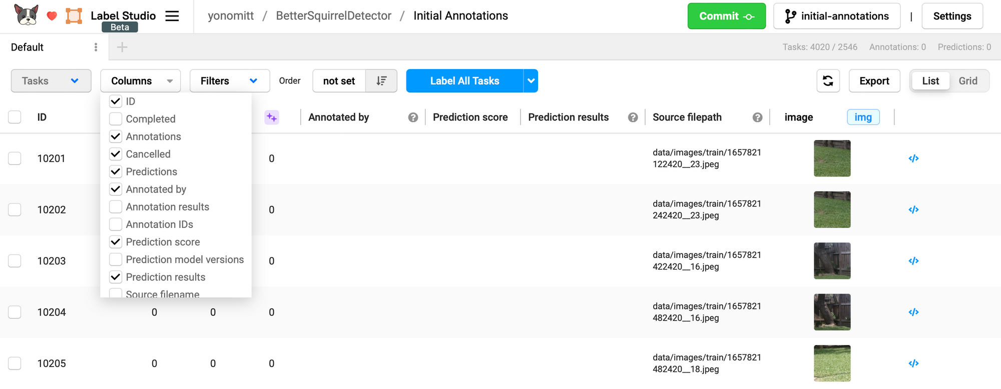
By default, predictions are not show in the list of tasks here. To change that, click the Columns drop-down menu and select Prediction score and Prediction results.

Based on the settings we chose, Label Studio will not call out to our server to make predictions until we ask it to. To do this, select all annotation tasks by clicking the check box next to the ID header. This will activate the Tasks drop-down menu.

Click the Tasks drop-down menu and select Retrieve Predictions. An alert box should appear asking you to confirm the action. Once you hit OK, Label Studio will start sending data to your server for predictions.

Now is a great time to get another cup of coffee, as this could take a while depending on how many tasks are available for prediction.

Conclusion

This is a good stopping point for part one of this tutorial. We’ve covered a lot of information here including:

• Serving a machine learning model behind a REST API
• Setting up a Label Studio project
• Connecting Label Studio to our REST API
• Running predictions on our unlabeled data

In the next part, we’ll be using these predictions to determine which data we want to label and then streaming just our labeled data to our training script. By doing this, we won’t have to download the entire database at once!

If you have any questions, feel free to reach out!