Tutorial: Reproducible Workflow for Tabular Data Hosted on Snowflake

In our previous blog, we explored how cloud-based data warehousing solutions like Snowflake can help organizations manage large amounts of data cost-effectively and at scale. Despite the benefits, reproducibility challenges may arise when working with complex data pipelines or mutable data.

To address this issue, we presented two versioning-based solutions. The first offer to version the query and metadata used to train the model, whereas the other also versions the queried data to achieve full reproducibility.

In this blog, we'll focus on implementing the second alternative using only open-source and free-tier solutions. To do so, we'll leverage the power of DagsHub and Snowflake, which offers an efficient way to version data and keep track of changes over time.

By using Snowflake as our cloud-based data warehousing solution, we'll demonstrate how you can store, query, and version data for reproducibility. Additionally, we'll follow the recommended GitFlow methodology for building fully reproducible machine learning projects.

By the end of this post, you will have gained a practical understanding of how to overcome reproducibility challenges in data management using versioning and cloud-based data warehousing solutions.

Setting up a database on Snowflake

In this project, we will use a dataset containing information about LEGO sets and their prices. This dataset is spread across several tables and includes data on themes, parts, categories, colors, production years, and prices of thousands of Lego sets in the market.

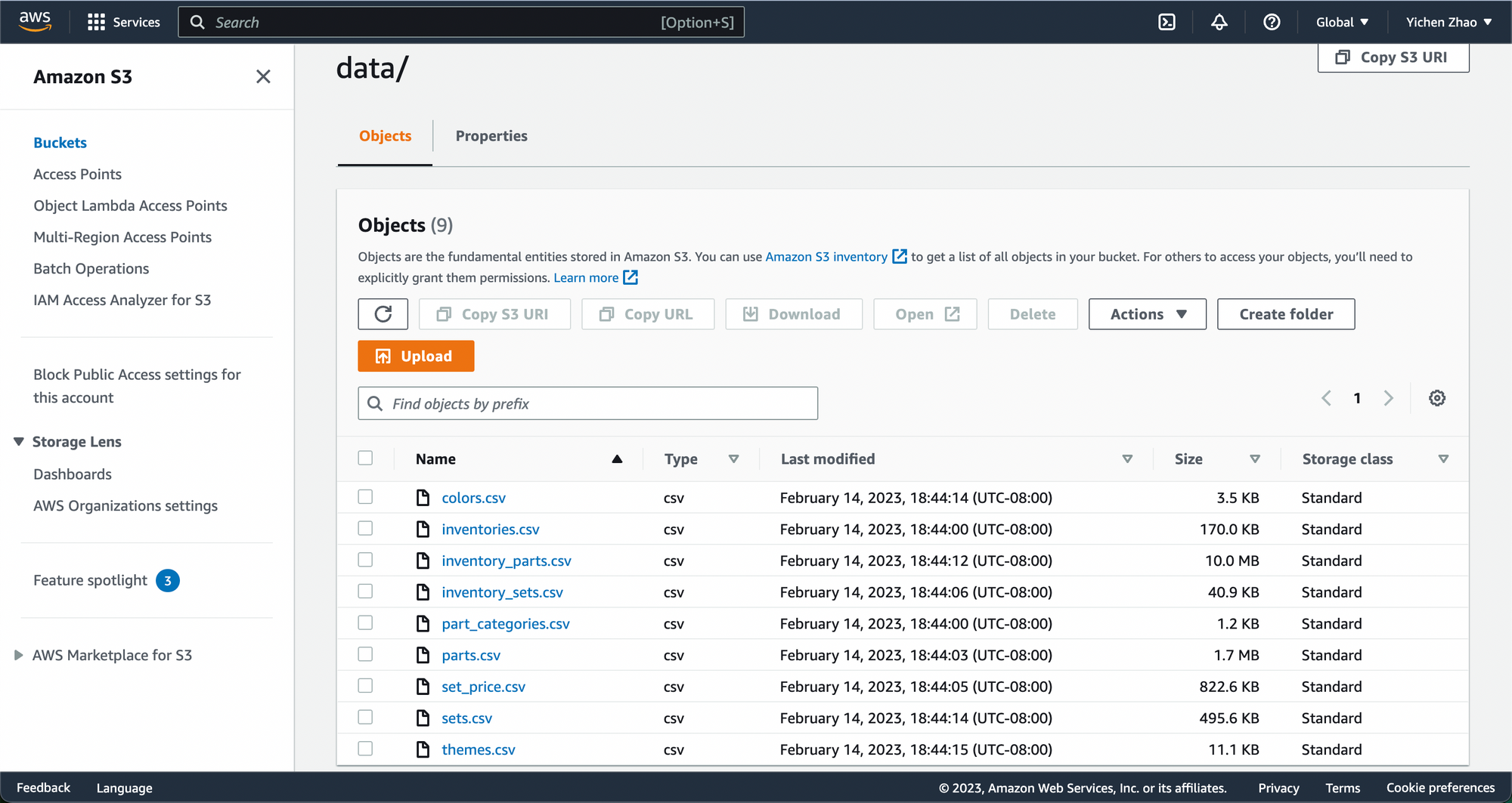
We host the database on Snowflake while storing the files on an AWS S3 bucket and granting Snowflake access to connect to the bucket.

While both Snowflake and AWS S3 support services of cloud-based data storage, Snowflake benefits users over vanilla S3 buckets with its built-in data warehouse functionalities. Snowflake is designed to be a cloud-based data warehouse, which means it has built-in support for SQL queries, indexing, and optimization. This makes it easier to perform complex queries and analyze large datasets without having to manage a separate data warehouse if we are to retrieve data from a vanilla S3 bucket.

A detailed guide on creating buckets and uploading files on AWS can be found here.

To build a Snowflake database using data files stored in an AWS S3 bucket, you need to configure your Snowflake account with AWS S3. This step includes granting Snowflake access permission to the files in your S3 bucket, creating a cloud storage integration in Snowflake, etc. Detailed documentation is available on Snowflake’s docs for you to follow along.

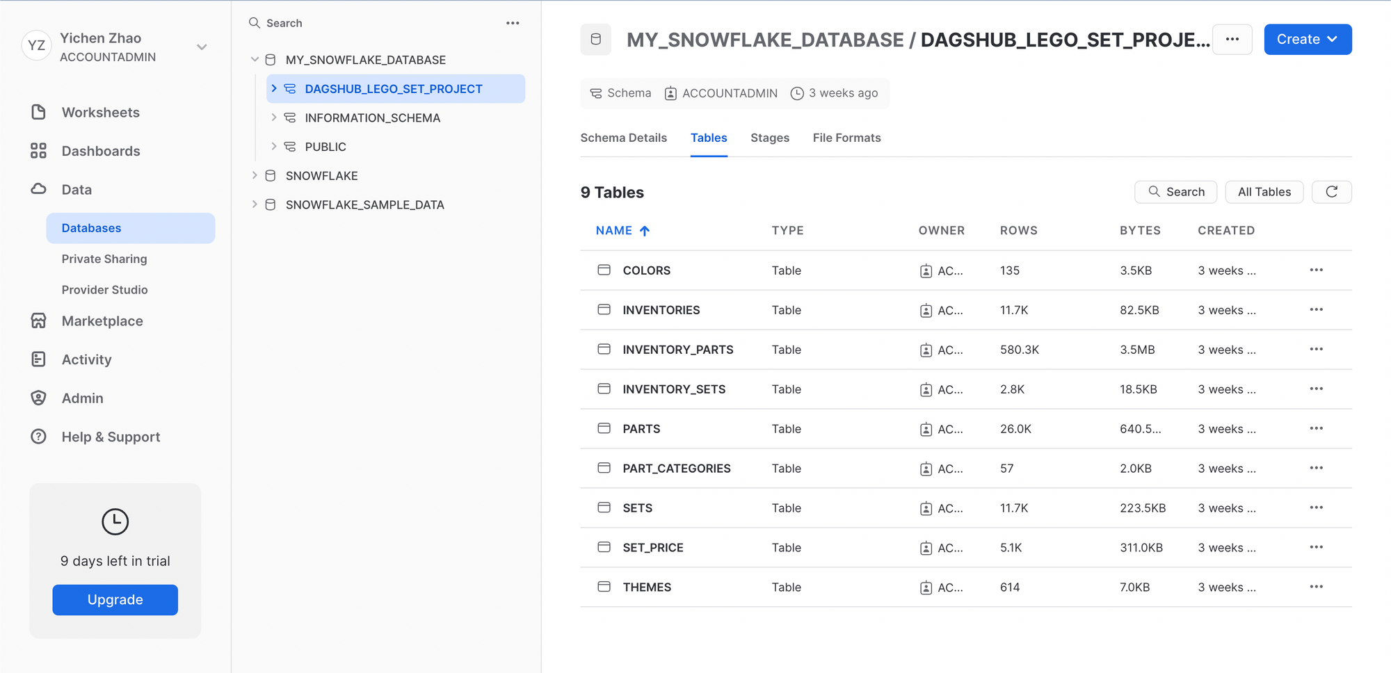
Completing the configurations using the above docs, we are able to import the data from the S3 bucket to the tables we create in our Snowflake database. This file contains the example code that configures my Snowflake database and imports data from the S3 bucket to Snowflake.

At the end my Snowflake database is named "dagshub_lego_set_project" whose structure looks like this:

Querying data from Snowflake database

Once you have a cloud database on Snowflake, you are able to access it any time when you need data for your machine learning project. A Python API called Snowflake Connector for Python can be used to connect your local machine to a Snowflake database and query data from there. A complete installation guide can be found here.

To successfully connect to your Snowflake database, you need the following list of information:

• Snowflake account username
• Snowflake account password
• Snowflake account ID
• Snowflake data warehouse name
• Snowflake database name
• Snowflake schema name

The API call then looks like this:

from snowflake.connector import connect

conn = connect(
        user=<my_username>,
        password=<my_password>,
        account=<my_account_id>, 
        warehouse=<my_warehouse>, 
        database=<my_database>, 
        schema=<my_schema>
    )

cursor = conn.cursor()

Full code for Snowflake connection using Python APIs can be examined here.

A cursor can be defined when making a connection to your Snowflake database. A cursor is a programming language construct in SQL that enables traversal over the records or rows in a database table. It allows the application to access and manipulate the data in a more granular way than simply executing a query that returns all the rows at once. With a cursor, the application can retrieve and process rows individually or in small batches, which can be more efficient for many use cases.

For predicting the price of a LEGO set, we need information mainly from two tables: SET_PRICE and THEMES. We then write SQL queries to retrieve data from both tables using the cursor and store the result tables into Pandas data frames.

The following provides a code snippet of querying data from SET_PRICE table and storing the result table as a data frame.

	SET_PRICE = '''
    SELECT set_price.id,
        set_price.name,
        set_price.category,
        set_price.year,
        set_price.parts,
        sets.theme_id,
        set_price.img_link,
        set_price.mean_price
    FROM set_price
            LEFT JOIN sets
                    ON set_price.id = sets.set_num
    WHERE mean_price <> 0;
'''

cursor.execute(SET_PRICE)

column_names = ['set_id', 'set_name', 'category', 'prod_year', 'num_parts', 'theme_id', 'img_link', 'price']
set_price_df = pd.DataFrame(cursor, columns=column_names)

Data Version Control for Reproducibility

Version control plays a crucial role in achieving reproducibility in machine learning projects. Version control systems, for all project components (code, data, models, experiments, etc.) help keep track of changes made over time and ensure that what was tracked can be reproduced at any point in time.

To achieve reproducibility for the dataset in this project, we utilize DagsHub tracking features to perform version control of the SQL queries and the result tables.

We collect all SQL queries into one .py file and use Git to track this file. On the other hand, since Pandas data frames themselves are hard to perform version control on, we save the data frames as CSV files in the repository and then use DVC to track these CSV files instead.

To save result tables as CSV files:

set_price_df.to_csv('../dataframes/lego_set_prices.csv')

then track these csv files with DVC in command lines:

dvc add ../dataframes/lego_set_prices.csv

You may ask at this point: why bother doing all these trackings?

When dealing with complex data pipelines in Snowflake or data that changes over time, it can be difficult to maintain lineage between the model and the data used to train it.

Although Snowflake provides some versioning capabilities such as Time Travel, these features come with certain limitations. For example, the community tier only allows users to travel back up to one day, while the enterprise edition only allows up to 90 days.

Additionally, queries may not be reproducible due to variations in query syntax or settings, leading to different results even with the same query. Further, changes made to the underlying code or database schema can also affect query reproducibility. In other words, it's not sufficient to simply version the query itself since not all queries are reproducible.

To achieve reproducibility and optimize model performance, it is essential to track the raw data used to train the model and the processing method conducted on it. For that, we’ll version the raw data with DVC and the code that process the data with Git and host them under the same Git commit. This way, when we can reproduce the results by simply reverting back to that Git commit.

Feature Engineering

With the SQL query shown above to get a result table from SET_PRICE, we find that two features cannot be utilized directly and thus need further actions. The theme_id feature records a very detailed classification of themes for each LEGO set. This can be problematic because a categorical feature with too many classes usually degrades the model's performance. Therefore, we trace the parent theme for each theme ID using information from the THEME table. This way we reduce the number of classes in the category feature to a manageable amount. Here is a code snippet that does the task described above, and full code can be examined here:

# find the raw theme of each theme id
def find_raw_theme(id):
    for i, raw_theme_id in enumerate(raw_theme_df.theme_id):
        if i == len(raw_theme_df) - 1 and id >= raw_theme_id:
            return raw_theme_df[raw_theme_df.theme_id == raw_theme_id].name.values[0]
        
        if i < len(raw_theme_df) - 1 and (id >= raw_theme_id and id < raw_theme_df.theme_id[i + 1]):
            return raw_theme_df[raw_theme_df.theme_id == raw_theme_id].name.values[0]

set_price_df['theme'] = set_price_df['theme_id'].apply(func=find_raw_theme)

The other feature that needs processing is img_link. It contains URLs that link to an image of each LEGO set. What we’d like to do here, is retrieve the image from the link and compute the average color in an RGB format of the image to examine the relationship between the price of a LEGO set and its overall color.

The code snippet that does this task is provided as follows, and the full code can be examined here:

# get the average RGB parameters from the lego set image
def img_to_rgb(img_url):
    '''Get the average RGB parameters of the given image.'''
    try:
        response = requests.get(img_url)
        img = Image.open(BytesIO(response.content))
    except:
        return np.array([-1, -1, -1])
    rgb = np.array(img).reshape((-1, 3))
    return np.mean(rgb, axis=0)

prepend = '<https://cdn.rebrickable.com/media/thumbs>'
set_price_df['r_avg'] = set_price_df['img_link'].apply(func=lambda x: img_to_rgb(prepend + x)[0])
set_price_df['g_avg'] = set_price_df['img_link'].apply(func=lambda x: img_to_rgb(prepend + x)[1])
set_price_df['b_avg'] = set_price_df['img_link'].apply(func=lambda x: img_to_rgb(prepend + x)[2])

Building the prediction model

We first load the data file that is stored and tracked in previous steps. This dataset contains information on the category, theme, publishing year, number of parts, and average set color in RGB format of each LEGO set, and we attempt to model these features against the price. The model we use here is the Lasso Regression model.

For tuning this Lasso regression model, we try a wide variety of values for the regularization penalty and choose the one that maximizes validation R2 score where the regularization penalty equals 0.0001, and evaluate the model performance on an independent test set. Finally, we get a R2 score of 0.487 on the test set by a Lasso regression model with regularization penalty being 0.0001.

What If We Use Different Data?

Now we wonder: what if we grab a different set of features from the database and use those features to train the model?

For instance, we try not to take the color of a LEGO set into consideration, and thus, do not need the information for the image link when querying data, i.e. not selecting “set_price.img_link” in the above SQL query “SET_PRICE”.

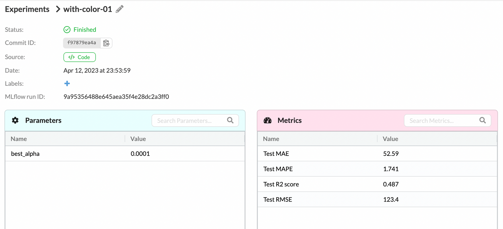
We update our result tables using this new SQL query. Then we retrain a Lasso regression model with the same dataset from above except that it now does not contain the average set color in RGB format for each LEGO set. By fine-tuning the regularization parameter of the Lasso model, we get R2 score, MAE, MAPE, and RMSE:

Under the “Experiments” tab on DagsHub, we could compare the two above experiments:

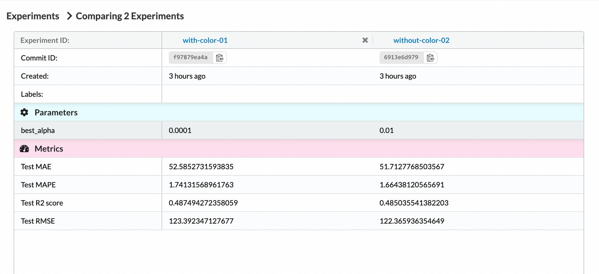
By comparing the test metrics, we can see that other than the R2 score, the experiment without the color features provides better results.

Reproduce the Experiment’s Results

Upon recognizing that the experiment not considering the color features yields better test results, the next step is to reproduce this particular experiment. This is where our workflow shines. Each experiment is associated to a commit ID which is assigned with versioning the data files. By encapsulating the version of all project components, we can easily revert the repo to retrieve the experiment that we desire by copying the commit ID and running the following command line:

git revert <commit_id>

This brings you back to the Git commit that stores the data frames, its SQL queries, and the model trained from those data frames which is proven to have the best model performance. From here you could further play around with the data frames of this particular version, reproduce the model with the best performance, or do whatever you would like to make further progress.

Conclusion

The use of version control in retrieving data from a cloud-based database is a critical step towards achieving reproducibility in building machine learning projects with a large database.  This project demonstrates the importance of version control in achieving reproducibility in a machine learning pipeline. By using Git and DVC to track and compare different data querying attempts, we can locate the version of the attempt that leads to the best model performance. This not only improves reliability of the model but also enables us to reproduce the results at any point in time.

Going through this blog post, you learned:

• about connecting an AWS S3 bucket to Snowflake
• how to access your data via a Snowflake connector Python API
• why and how to version control your data queries using Git and the processed data tables using DVC
• how to compare multiple SQL queries for better model performance and realize reproducibility using version control system

The DagsHub repository where I host this project can be accessed through here. You are more than welcome to go through the repository thoroughly for any details that interest you.